Single-channel analysis tutorial
This tutorial walks through a complete 2D single-channel CellColoc workflow based on the interactive Jupyter notebook
user_scripts/nb_dapi_stained_nuclei_2D_single_channel_user_script.ipynb,
which is identical to the interactive Python script
user_scripts/dapi_stained_nuclei_2D_single_channel_user_script.py,
which you can use alternatively if you prefer the VS Code interactive window workflow.
The goal is to show how to analyze a one-channel 2D microscopy image from scratch when no colocalization step is needed and the main biological question is simply: how many segmented objects are present, how large are they, and what is their morphology?
This tutorial uses the single-channel CellColoc workflow, which reuses the same segmentation backends and interactive mechanics as the multi-channel pipeline, but skips all marker-overlap logic.
Dataset used in this tutorial
The tutorial uses the example dataset dapi_stained_nuclei_2D.ome.tif of
DAPI-stained nuclei originally published by Raissa Rathar on
Zenodo. This dataset is included
in the CellColoc example data collection. Please download it from Zenodo as
described in the Example data set section
first if you want to follow along with the tutorial. Store the downloaded
example dataset locally at a convenient location. For the remainder of this
tutorial, we assume that you have placed it in a folder called
example_data/ relative to your current working directory/current example
script:
example_data/dapi_stained_nuclei_2D/dapi_stained_nuclei_2D.ome.tif
This is a true 2D OME-TIFF file with two channels. In this tutorial, we do not use both channels for a colocalization analysis. Instead, we deliberately pick just one channel and count its segmented nuclei-like objects.
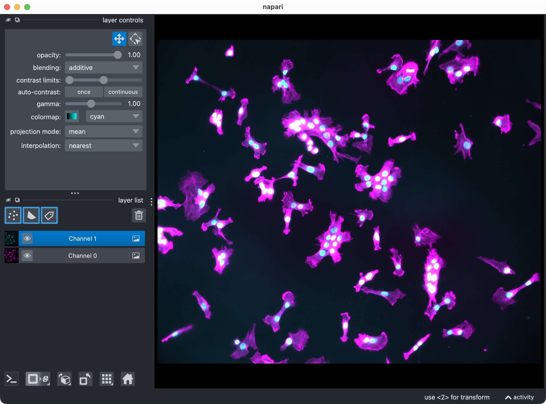
The DAPI-stained nuclei example dataset shown in napari with the two raw channels.
In this tutorial, the single-channel workflow is configured so that:
channel_index=1is loaded and segmented,the segmented objects are interpreted as DAPI-stained nuclei,
no second marker channel is used.
The same structure can be reused for any other one-channel or one-target use case, for example:
counting nuclei in one DAPI channel,
segmenting one soma channel only,
counting puncta or aggregates in a single fluorescence channel,
measuring ROI-wise occupancy of one segmented structure.
How to use this tutorial
The associated user-script
user_scripts/nb_dapi_stained_nuclei_2D_single_channel_user_script.ipynb
is organized in cells, reflecting the structure of this tutorial. The same
applies to the alternative Python script (there: # %% cells)
user_scripts/dapi_stained_nuclei_2D_single_channel_user_script.py.
The recommended way to follow this tutorial is:
open
user_scripts/nb_dapi_stained_nuclei_2D_single_channel_user_script.ipynboruser_scripts/dapi_stained_nuclei_2D_single_channel_user_script.py,run the cells from top to bottom,
adjust only the configuration values that are relevant for your own data.
The subsections below follow the same order as the script cells.
Imports
The first cell imports the public single-channel CellColoc API, napari, NumPy,
and dataclasses.replace:
from dataclasses import replace
from pathlib import Path

import napari
import numpy as np

from cellcoloc import (
    CellposeModelConfig,
    RuntimeConfig,
    SingleChannelAnalysisConfig,
    SingleChannelConfig,
    SingleChannelDisplayNames,
    analyze_existing_single_channel_masks,
    create_full_image_roi_labels,
    create_single_channel_roi_drawing_viewer,
    export_single_channel_outputs,
    extract_single_channel_masks_from_viewer,
    load_roi_labels,
    load_single_channel_image,
    prepare_loaded_single_channel_image_for_analysis,
    refine_single_channel_run_result_from_cellpose_cache,
    run_roi_single_channel_segmentation,
    save_roi_labels_from_shapes,
    show_single_channel_results,
    try_load_single_channel_roi_labels)

PROJECT_ROOT = Path(__file__).resolve().parents[1]
What this cell does:
locates the repository root via
PROJECT_ROOT,imports the single-channel configuration dataclasses and helper functions,
imports napari for ROI drawing and result inspection,
imports
replaceso that temporary refinement configs can be derived from the base segmentation config without overwriting it.
Project settings
The next cell contains the complete single-channel analysis configuration:
DATA_PATH = PROJECT_ROOT / "example_data" / "dapi_stained_nuclei_2D" / "dapi_stained_nuclei_2D.ome.tif"

CHANNEL_CONFIG = SingleChannelConfig(
    channel_index=1)

DISPLAY_NAMES = SingleChannelDisplayNames(
    channel="DAPI",
    objects="Segmented DAPI nuclei")

VOXEL_SCALE_ZYX = (0.325, 0.325)

MODEL_CONFIG = CellposeModelConfig(
    model_name_or_path="cpsam",
    segmentation_method="cellpose",
    diameter=None,
    do_3d=None,
    z_crop=None,
    z_projection=None,
    anisotropy=False,
    flow3d_smooth=0,
    prefilter=None,
    postfilters=None,
    cellprob_threshold=0.0,
    flow_threshold=0.4)

ANALYSIS_CONFIG = SingleChannelAnalysisConfig(
    min_object_voxels=50)

RUNTIME_CONFIG = RuntimeConfig(
    draw_rois=True,
    process_rois=True,
    open_results=True,
    use_gpu=True,
    crop_for_testing=None,
    image_loading_mode="memory")

USE_FULL_IMAGE_AS_SINGLE_ROI = True
REUSE_EXISTING_ROI_MASK_IF_AVAILABLE = True
INITIAL_RESULT_LAYER_KEYS = [
    "channel_image",
    "rois",
    "roi_numbers",
    "masks"]
REFINEMENT_RESULT_LAYER_KEYS = [
    "masks",
    "rois"]

existing_roi_labels = None
result_viewer = None
This is the most important cell for adapting the tutorial to your own data.
Data path
DATA_PATH points to the microscopy file that should be analyzed.
Replace this with your own OME-TIFF, CZI, or other OMIO-readable dataset when you adapt the workflow.
Single-channel assignment
CHANNEL_CONFIG is now a SingleChannelConfig instead of the usual
two-channel ChannelConfig.
The key setting is:
channel_index=1
This means: load only the raw channel at index 1 and pass it into the single-channel segmentation workflow.
Display names
DISPLAY_NAMES is now a SingleChannelDisplayNames config. It controls:
the name of the image layer in napari,
the name of the segmentation label layer.
For your own projects, choose biologically meaningful names such as
"DAPI", "Nuclei", "Neuronal somata", or "Aggregates".
Voxel scale
VOXEL_SCALE_ZYX defines the physical size of voxels or pixels as
(z, y, x). For true 2D data, CellColoc also accepts a shorter
(y, x) tuple, which is exactly what is used here:
VOXEL_SCALE_ZYX = (0.325, 0.325)
Internally, this is expanded to (1.0, 0.325, 0.325).
You can also set this to None and let CellColoc try to resolve it from
OMIO metadata.
Segmentation config
MODEL_CONFIG contains the segmentation settings for the single analyzed
channel.
In this tutorial, the single channel uses Cellpose:
segmentation_method="cellpose"
Important options are the same as in the multi-channel workflow:
model_name_or_path: built-in model name such as"cpsam"or a custom model path.segmentation_method: one of"cellpose","otsu","li", or"percentile".diameter: optional object diameter for Cellpose.Nonelets newer Cellpose infer the scale automatically.cellprob_thresholdandflow_threshold: Cellpose threshold parameters.prefilter: optional image prefiltering before segmentation.postfilters: optional mask cleanup after segmentation.z_cropandz_projection: available here as well, even though this particular tutorial uses a true 2D dataset.
If you prefer a threshold-based workflow, you can switch to:
segmentation_method="otsu"
or one of the other supported non-Cellpose backends.
Analysis config
ANALYSIS_CONFIG is a SingleChannelAnalysisConfig.
For now, its key parameter is:
min_object_voxels: discard segmented objects smaller than this size before counting and table generation.
Runtime settings
RUNTIME_CONFIG controls runtime behavior rather than segmentation logic.
Important options are:
draw_rois: whether napari-based ROI drawing is enabled.open_results: whether result visualization is shown in napari.use_gpu: whether Cellpose should try to use a GPU.crop_for_testing: optional temporary crop for debugging or fast prototyping.image_loading_mode:"memory"or"memap".
Whole-image versus ROI mode
Two additional switches control whether the full 2D image is analyzed directly or whether custom ROIs are used:
USE_FULL_IMAGE_AS_SINGLE_ROI = TrueREUSE_EXISTING_ROI_MASK_IF_AVAILABLE = True
For this tutorial, the default assumption is whole-image analysis.
If you prefer ROI-based analysis instead:
set
USE_FULL_IMAGE_AS_SINGLE_ROI = False,keep
RUNTIME_CONFIG.draw_rois = Trueto draw new ROIs,or keep
REUSE_EXISTING_ROI_MASK_IF_AVAILABLE = Trueto reuse a saved ROI mask from a previous run.
Load the analysis channel
The next cell loads the configured analysis channel from disk:
loaded_image = load_single_channel_image(
    source_path=DATA_PATH,
    channel_config=CHANNEL_CONFIG,
    voxel_scale_zyx=VOXEL_SCALE_ZYX,
    crop_for_testing=RUNTIME_CONFIG.crop_for_testing,
    image_loading_mode=RUNTIME_CONFIG.image_loading_mode)
loaded_image = prepare_loaded_single_channel_image_for_analysis(
    loaded_image,
    MODEL_CONFIG)
print(f"Results directory:\n{loaded_image.paths.results_dir}")

if REUSE_EXISTING_ROI_MASK_IF_AVAILABLE:
    existing_roi_labels = try_load_single_channel_roi_labels(loaded_image.paths.roi_mask_path)
This step:
reads the microscopy file through OMIO,
extracts the configured analysis channel only,
resolves voxel size,
creates standardized output paths inside the dataset’s
results/directory,optionally prepares the image for z projection if that feature is enabled.
Because this tutorial uses a plain 2D dataset, the loaded analysis view stays 2D throughout.
Optional: Draw ROIs interactively in napari
The next cell only becomes relevant when you disable whole-image mode:
if USE_FULL_IMAGE_AS_SINGLE_ROI:
    print("Whole-image mode is enabled. ROI drawing is skipped.")
elif existing_roi_labels is not None:
    print("An existing ROI mask was found and will be reused. ROI drawing is skipped.")
elif RUNTIME_CONFIG.draw_rois:
    roi_viewer, shapes_layer = create_single_channel_roi_drawing_viewer(
        loaded_image=loaded_image,
        display_names=DISPLAY_NAMES)
    print("Draw ROIs in napari and close the window. Then run the next cell.")
    napari.run()
else:
    print("ROI drawing is disabled. The next cell will load an existing ROI mask from disk.")
The logic is:
if
USE_FULL_IMAGE_AS_SINGLE_ROIisTrue, ROI drawing is skipped,else, if
REUSE_EXISTING_ROI_MASK_IF_AVAILABLEisTrue, CellColoc first looks for a previously saved ROI label mask in the results directory,if such a saved ROI mask exists, it is reused and drawing is skipped,
if not, napari opens and you can draw one or more ROIs interactively.
This is the same ROI logic used in the multi-channel scripts, just applied to the single analyzed channel.
Optional: Save drawn ROIs or load an existing ROI mask
The following cell resolves the final ROI mask that will be used for analysis:
if USE_FULL_IMAGE_AS_SINGLE_ROI:
    roi_labels_2d = create_full_image_roi_labels(loaded_image.image.shape[1:])
elif existing_roi_labels is not None:
    roi_labels_2d = existing_roi_labels
elif RUNTIME_CONFIG.draw_rois:
    roi_labels_2d = save_roi_labels_from_shapes(
        shapes_layer=shapes_layer,
        output_path=loaded_image.paths.roi_mask_path,
        image_shape_yx=loaded_image.image.max(axis=0).shape,
        scale_yx=loaded_image.voxel_scale_zyx[1:])
else:
    roi_labels_2d = load_roi_labels(loaded_image.paths.roi_mask_path)

roi_ids = np.unique(roi_labels_2d)
roi_ids = roi_ids[roi_ids != 0]
print(f"ROI ids: {roi_ids}")
This cell supports three modes:
Whole-image mode
If USE_FULL_IMAGE_AS_SINGLE_ROI is True, CellColoc creates one ROI
that spans the complete image.
Interactive ROI mode
If whole-image mode is disabled and you drew ROIs in napari, the shapes are rasterized into a label image and saved to the results directory.
Saved ROI reuse mode
If a saved ROI mask was found earlier, that existing label image is loaded and used directly.
After this step, roi_labels_2d contains the actual ROI label map for the
analysis, and the script prints the detected ROI IDs.
Run the ROI-wise single-channel segmentation and counting
This is the main analysis step:
run_result = run_roi_single_channel_segmentation(
    loaded_image=loaded_image,
    roi_labels_2d=roi_labels_2d,
    model_config=MODEL_CONFIG,
    analysis_config=ANALYSIS_CONFIG,
    runtime_config=RUNTIME_CONFIG,)
print("Single-channel analysis finished. "
      f"Overview rows: {len(run_result.tables.overview)}, "
      f"object rows: {len(run_result.tables.objects)}.")
What happens here:
each ROI is processed separately,
the single analysis channel is segmented according to
MODEL_CONFIG,small objects are filtered according to
ANALYSIS_CONFIG,object-wise and ROI-wise result tables are assembled.
The function returns a run_result object that contains:
the full label mask,
per-object and per-ROI tables,
optional Cellpose refinement cache data.
Depending on the image size, ROI count, and available hardware, this step can take some time. For quick testing, you can use:
RUNTIME_CONFIG.crop_for_testing = (slice(0, 1), slice(0, 512), slice(0, 512))
Visualize the result in napari
The next cell opens the current result in napari:
if RUNTIME_CONFIG.open_results:
    result_viewer = show_single_channel_results(
        loaded_image=loaded_image,
        roi_labels_2d=roi_labels_2d,
        run_result=run_result,
        display_names=DISPLAY_NAMES,
        viewer=result_viewer,
        layers_to_show=INITIAL_RESULT_LAYER_KEYS,
        replace_existing_layers=True)
    print("Inspect the single-channel result in napari and close the window when finished.")
    napari.run()
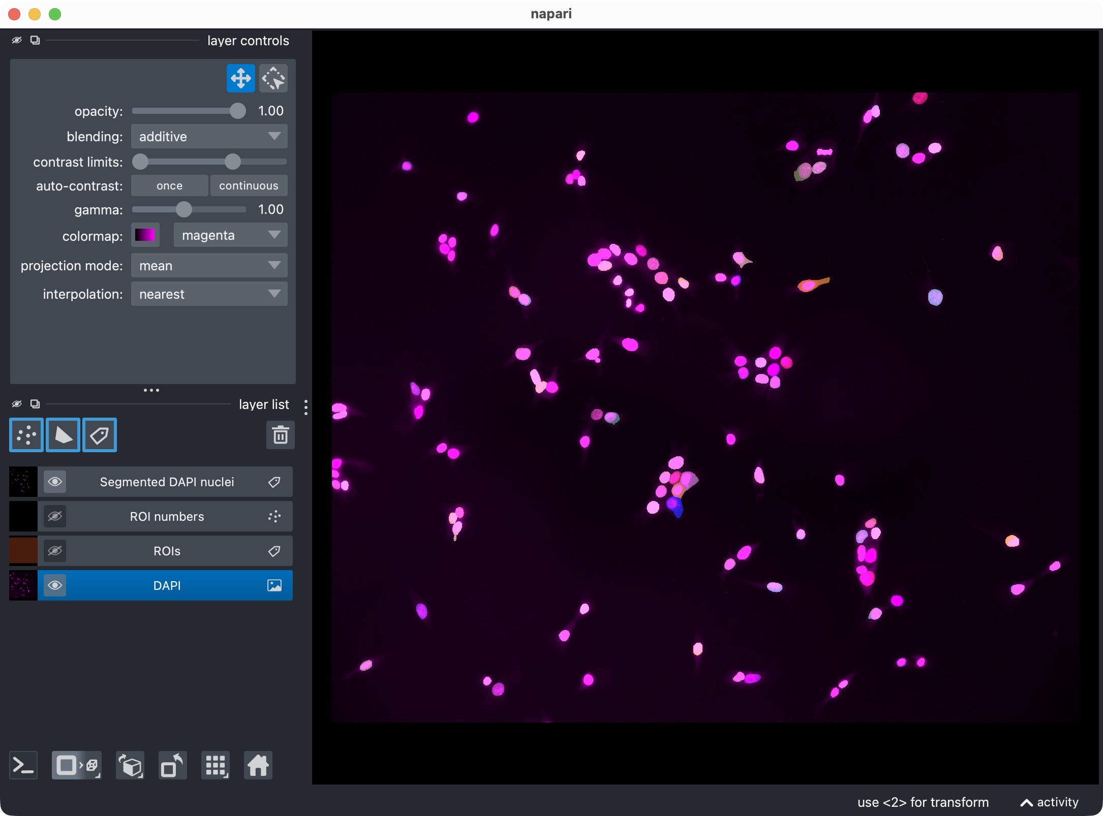
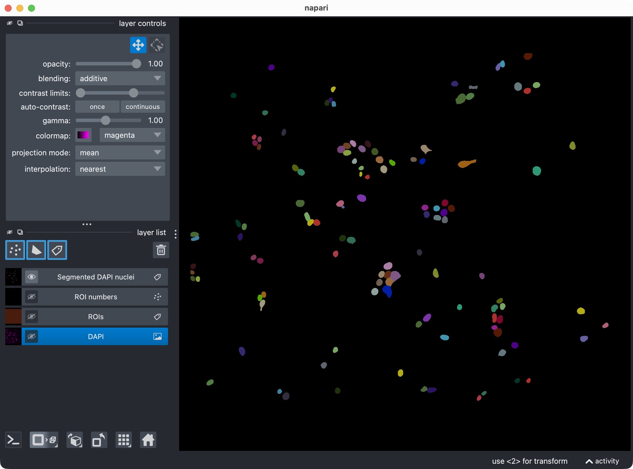
Segmentation result of the single-channel workflow, showing the DAPI-stained nuclei and the resulting segmentation layer of the nuclei (top) and the segmentation layer only (bottom).
This visualization usually includes:
the analysis channel,
the ROI labels,
the segmented object masks.
This is the first checkpoint where you inspect whether the segmentation looks plausible before refining anything.
If you want to skip napari output during batch-style testing, set:
RUNTIME_CONFIG.open_results = False
Optional: Refine Cellpose thresholds and inspect the updated result
The next cell performs cache-based post hoc refinement:
REFINE_WITH_CACHED_CELLPOSE_OUTPUTS = False
REFINEMENT_ANALYSIS_Z_CROP = None

REFINED_CELLPROB_THRESHOLD = MODEL_CONFIG.cellprob_threshold - 2.0
REFINED_FLOW_THRESHOLD = MODEL_CONFIG.flow_threshold

REFINED_POSTFILTERS = None
REFINED_MIN_INTENSITY_MEASURE = "mean"
REFINED_MIN_INTENSITY_THRESHOLD = None
REFINED_LOCAL_CONTRAST_K = 1.0
REFINED_LOCAL_CONTRAST_SHELL_INNER_RADIUS = 1.0
REFINED_LOCAL_CONTRAST_SHELL_OUTER_RADIUS = 4
REFINED_BRIGHT_PIXEL_MEASURE = "count"
REFINED_BRIGHT_PIXEL_THRESHOLD = None
REFINED_BRIGHT_PIXEL_MIN_COUNT = None
REFINED_BRIGHT_PIXEL_MIN_FRACTION = None

effective_refinement_z_crop = (
    MODEL_CONFIG.z_crop if REFINEMENT_ANALYSIS_Z_CROP is None else REFINEMENT_ANALYSIS_Z_CROP)

if REFINE_WITH_CACHED_CELLPOSE_OUTPUTS:
    refined_model_config = replace(
        MODEL_CONFIG,
        z_crop=effective_refinement_z_crop,
        postfilters=REFINED_POSTFILTERS,
        min_intensity_measure=REFINED_MIN_INTENSITY_MEASURE,
        min_intensity_threshold=REFINED_MIN_INTENSITY_THRESHOLD,
        local_contrast_k=REFINED_LOCAL_CONTRAST_K,
        local_contrast_shell_inner_radius=REFINED_LOCAL_CONTRAST_SHELL_INNER_RADIUS,
        local_contrast_shell_outer_radius=REFINED_LOCAL_CONTRAST_SHELL_OUTER_RADIUS,
        bright_pixel_measure=REFINED_BRIGHT_PIXEL_MEASURE,
        bright_pixel_threshold=REFINED_BRIGHT_PIXEL_THRESHOLD,
        bright_pixel_min_count=REFINED_BRIGHT_PIXEL_MIN_COUNT,
        bright_pixel_min_fraction=REFINED_BRIGHT_PIXEL_MIN_FRACTION)

    run_result = refine_single_channel_run_result_from_cellpose_cache(
        loaded_image=loaded_image,
        roi_labels_2d=roi_labels_2d,
        run_result=run_result,
        analysis_config=ANALYSIS_CONFIG,
        model_config=refined_model_config,
        cellprob_threshold=REFINED_CELLPROB_THRESHOLD,
        flow_threshold=REFINED_FLOW_THRESHOLD)

    print("Refined single-channel analysis finished. "
          f"Overview rows: {len(run_result.tables.overview)}, "
          f"object rows: {len(run_result.tables.objects)}.")

    result_viewer = show_single_channel_results(
        loaded_image=loaded_image,
        roi_labels_2d=roi_labels_2d,
        run_result=run_result,
        display_names=DISPLAY_NAMES,
        viewer=result_viewer,
        layers_to_show=REFINEMENT_RESULT_LAYER_KEYS,
        replace_existing_layers=True)
    print("Inspect the refined single-channel result in napari and close the window when finished.")
    napari.run()
else:
    print("Cached Cellpose refinement is disabled for this run.")
This step is useful when the initial Cellpose result is close to correct but slightly too permissive or too conservative.
The refinement works by rebuilding masks from cached Cellpose network outputs instead of rerunning the full network forward pass. This is much faster than launching a fresh segmentation from scratch.
Relevant refinement settings include:
REFINE_WITH_CACHED_CELLPOSE_OUTPUTS: enable or disable the refinement step.REFINED_CELLPROB_THRESHOLD: new Cellpose probability threshold for the single analyzed channel.REFINED_FLOW_THRESHOLD: new Cellpose flow threshold.REFINED_POSTFILTERS: optional post hoc filters such as"min_intensity","local_contrast", or"bright_pixel_support".
Optional: Reanalyze manually edited label layers from napari
The next cell supports a manual correction workflow:
REANALYZE_EDITED_LABELS_FROM_VIEWER = False

if REANALYZE_EDITED_LABELS_FROM_VIEWER:
    masks_from_viewer = extract_single_channel_masks_from_viewer(
        result_viewer,
        object_layer_name=DISPLAY_NAMES.objects)
    run_result = analyze_existing_single_channel_masks(
        loaded_image=loaded_image,
        roi_labels_2d=roi_labels_2d,
        masks=masks_from_viewer,
        analysis_config=ANALYSIS_CONFIG,
        analysis_z_bounds=run_result.analysis_z_bounds,
        refinement_context=run_result.refinement_context)

    result_viewer = show_single_channel_results(
        loaded_image=loaded_image,
        roi_labels_2d=roi_labels_2d,
        run_result=run_result,
        display_names=DISPLAY_NAMES,
        viewer=result_viewer,
        layers_to_show=REFINEMENT_RESULT_LAYER_KEYS,
        replace_existing_layers=True)
    print("Inspect the relabeled single-channel result in napari and close the window when finished.")
    napari.run()
else:
    print("Manual label reanalysis from the napari viewer is disabled for this run.")
This is useful when:
Cellpose split one object into several labels,
Cellpose merged neighboring objects incorrectly,
you want to remove or redraw objects directly in napari.
The workflow is:
inspect the result in napari,
edit the label layer manually,
run this cell,
let CellColoc recompute the tables from the updated mask layer.
The underlying image is not resegmented here. Instead, the edited label layer is read back from napari and analyzed as the new truth for this run.
Export results
The final cell exports the result tables and masks:
export_single_channel_outputs(
    run_result=run_result,
    paths=loaded_image.paths)
print("Final single-channel results exported.")
This writes the single-channel outputs to the dataset’s results/
directory.
The Excel workbook produced by the single-channel workflow contains three sheets:
object_summaryvoxel_plausibility_checkroi_overview
Result table: object_summary
This is the main biologically relevant per-object table. It contains one row per segmented object.
Identity and location columns
roi_idID of the ROI containing the object.
object_labelInteger label of the object in the exported segmentation mask.
centroid_z,centroid_y,centroid_xCoordinates of the object centroid. For true 2D data,
centroid_zis typically0.0because CellColoc internally represents 2D images as a singleton-z volume(1, Y, X).
2D morphology columns
For 2D or z-projected analyses, the following columns are populated:
object_area_px_2dObject area in pixels.
object_area_um2_2dObject area in square micrometers.
object_perimeter_px_2dObject perimeter in pixels.
object_perimeter_um_2dObject perimeter converted to micrometers.
object_roundness_2dClassical 2D roundness
\[\mathrm{roundness} = \frac{4 \pi A}{P^2}\]where \(A\) is the object area and \(P\) is its perimeter. Values closer to
1indicate a more circular object.object_eccentricity_2dEccentricity of the ellipse fitted to the object. Values near
0indicate a round object, while values near1indicate a strongly elongated one.
3D morphology columns
For true 2D analyses, the 3D-specific columns are present but remain empty
(NaN). They become relevant for true 3D single-channel workflows:
object_volume_voxels_3dObject volume in voxels.
object_volume_um3_3dObject volume in cubic micrometers.
object_surface_area_um2_3dVoxel-based estimate of the object surface area in square micrometers.
object_sphericity_3d3D sphericity estimate. Values closer to
1indicate a shape more similar to a sphere.object_ellipticity_3dSimple elongation score derived from the object’s coordinate spread in 3D. Higher values indicate more anisotropic or elongated shapes.
Result table: voxel_plausibility_check
This sheet is mainly technical. It is a consistency check that compares two ways of counting object voxels.
roi_idID of the ROI containing the object.
object_labelInteger label of the object in the segmentation mask.
object_voxelsDirect voxel or pixel count of the object from the mask.
object_voxels_propsThe same size computed by
skimage.regionprops.object_voxels - object_voxels_propsDifference between the two counting methods.
In ordinary runs this difference should be 0. Non-zero values would
indicate an unexpected inconsistency between direct mask counting and
regionprops-based measurement.
Result table: roi_overview
This table contains one row per ROI and summarizes object counts, occupancies, and per-ROI mean morphology values.
ROI identity and size
roi_idInteger ID of the ROI.
n_objectsNumber of segmented objects in this ROI.
drawn_roi_area_pxROI area in pixels.
drawn_roi_area_um2ROI area in square micrometers.
roi_volume_voxelsROI size in voxels. For true 2D data this corresponds to one z slice.
roi_volume_um3ROI size in cubic micrometers.
Occupancy columns
These columns describe how much of the ROI is occupied by segmented objects.
object_occupancy_area_px_2d_projectionNumber of ROI pixels covered by at least one object in 2D.
object_occupancy_area_um2_2d_projectionSame occupancy area converted to square micrometers.
object_occupancy_coverage_2d_percentPercentage of the ROI area covered by objects in 2D.
object_occupancy_volume_voxels_3dNumber of occupied voxels in the full analysis volume.
object_occupancy_volume_um3_3dSame occupancy converted to cubic micrometers.
object_occupancy_coverage_3d_percentPercentage of the ROI volume covered by objects.
Average morphology columns
The remaining columns start with average_ and report per-ROI means of the
corresponding object-summary metrics.
For example:
average_object_area_px_2dMean object area in pixels across all objects in the ROI.
average_object_area_um2_2dMean object area in square micrometers.
average_object_perimeter_px_2dMean object perimeter in pixels.
average_object_perimeter_um_2dMean object perimeter in micrometers.
average_object_roundness_2dMean 2D roundness of the objects in the ROI.
average_object_eccentricity_2dMean 2D eccentricity of the objects in the ROI.
average_object_volume_voxels_3dMean object volume in voxels for true 3D workflows.
average_object_volume_um3_3dMean object volume in cubic micrometers for true 3D workflows.
average_object_surface_area_um2_3dMean object surface area in square micrometers for true 3D workflows.
average_object_sphericity_3dMean object sphericity for true 3D workflows.
average_object_ellipticity_3dMean object ellipticity-like elongation score for true 3D workflows.
For a pure 2D analysis such as this tutorial, the 3D-average columns are
typically present but remain empty (NaN), whereas the 2D-average columns
carry the relevant morphology information.