2D data analysis tutorial

This tutorial walks through a complete 2D CellColoc workflow based on the interactive Jupyter notebook

user_scripts/nb_dapi_stained_nuclei_2D_user_script.ipynb,

which is identical to the interactive Python script

user_scripts/dapi_stained_nuclei_2D_user_script.py,

which you can use alternatively if you prefer the VS Code interactive window workflow.

The goal is to show how to analyze a two-channel 2D microscopy image from scratch, how to configure CellColoc for whole-image analysis, and how to optionally switch to ROI-based analysis when needed.

Dataset used in this tutorial

The tutorial uses the example dataset dapi_stained_nuclei_2D.ome.tif of DAPI-stained nuclei originally published by Raissa Rathar on Zenodo. This dataset is included in the CellColoc example data collection. Please download it from Zenodo as described in the Example data set section first if you want to follow along with the tutorial. Store the downloaded example dataset locally at a convenient location. For the remainder of this tutorial, we assume that you have placed it in a folder called example_data/ relative to your current working directory/current example script:

example_data/dapi_stained_nuclei_2D/dapi_stained_nuclei_2D.ome.tif

This is a true 2D OME-TIFF file with two channels. The file does not provide reliable biological channel names in the OME metadata, so the channel meaning is assigned explicitly in the script.

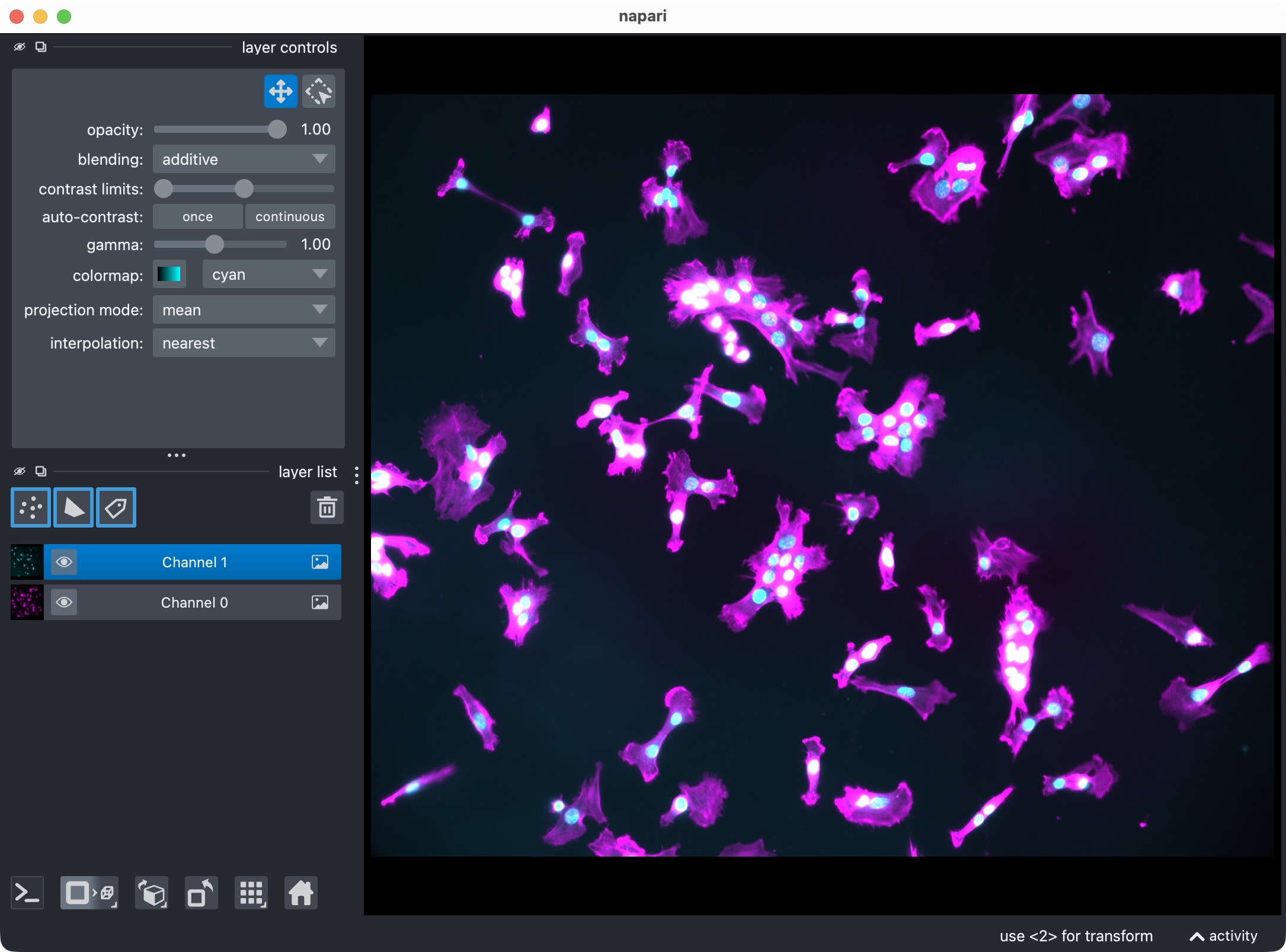
The DAPI-stained nuclei example dataset shown in napari with the two channels.

In this tutorial, we treat:

• channel 0 as the primary cell channel,

• channel 1 as the primary marker channel.

The same structure can be reused for any other 2D two-channel dataset by adapting the path, channel assignment, display names, and segmentation settings.

How to use this tutorial

The associated user-script

user_scripts/nb_dapi_stained_nuclei_2D_user_script.ipynb

is organized in cells, reflecting the structure of this tutorial. The same accounts for the alternative Python script (there: # %% cells)

user_scripts/dapi_stained_nuclei_2D_user_script.py.

The recommended way to follow this tutorial is:

1. open user_scripts/nb_dapi_stained_nuclei_2D_user_script.ipynb or user_scripts/dapi_stained_nuclei_2D_user_script.py,

2. run the cells from top to bottom,

3. adjust only the configuration values that are relevant for your own data.

The subsections below follow the same order as the script cells.

Imports

The first cell imports the public CellColoc API, napari, and NumPy:

# get the project root for accessing the example dataset which is 
# located in the parent folder of the user_scripts folder:
from pathlib import Path
PROJECT_ROOT = Path(__file__).resolve().parents[1]

# import relevant CellColoc functions for this script:
from cellcoloc import (
    analyze_existing_masks,
    CellposeModelConfig,
    ChannelConfig,
    ColocalizationConfig,
    DisplayNames,
    RuntimeConfig,
    create_full_image_roi_labels,
    create_roi_drawing_viewer,
    extract_label_masks_from_viewer,
    export_analysis_outputs,
    load_analysis_images,
    load_roi_labels,
    refine_run_result_from_cellpose_cache,
    run_roi_cellpose_colocalization,
    save_roi_labels_from_shapes,
    show_analysis_results,
    try_load_roi_labels)

# additional packages:
import napari
import numpy as np

What this cell does:

• locates the repository root via PROJECT_ROOT,

• imports the configuration dataclasses and helper functions from cellcoloc,

• imports napari for ROI drawing and result inspection.

Project settings

The next cell contains the complete analysis configuration:

# define path to the dataset file relative to the project root:
DATA_PATH = PROJECT_ROOT / "example_data" / "dapi_stained_nuclei_2D" / "dapi_stained_nuclei_2D.ome.tif"

# define the channel configuration for this dataset:
CHANNEL_CONFIG = ChannelConfig(
    cell_channel=0,
    marker_channel=1,
    optional_region_channel=None)

# define display names for the channels and result layers:
DISPLAY_NAMES = DisplayNames(
    cell="Channel 0",
    marker="Channel 1",
    optional_region="Unused",
    positive_cells="Channel 0 + Channel 1 positive masks")

# optional: define the voxel scale in ZYX (for 3D) or YX (for 2D) order. 
# Set this to None to use the voxel scale from the OME metadata, if available.
#VOXEL_SCALE_ZYX = (1.0, 0.325, 0.325) # CellColoc allows both ZYX and YX even for 2D data. 
VOXEL_SCALE_ZYX = (0.325, 0.325)

# define the Cellpose model configuration for the cell and marker segmentation:
CELL_MODEL_CONFIG = CellposeModelConfig(
    model_name_or_path="cpsam",     # 'cpsam' for cellpose 4, 'cty3', 'cyto2' or 'nuclei' for cellpose 3
    segmentation_method="cellpose", # 'cellpose' or: 'otsu', 'li', or 'percentile' for marker segmentation
    diameter=None,                  # if None, Cellpose will estimate the diameter from the data. Adjust if you know the expected cell/nuclei size in pixels.
    do_3d=None,                     # whether Cellpose should run in 3D mode; set to None to let CellColoc decide based on the input data shape
    cellprob_threshold=-0.5, # threshold for the cell probability map, between -6 and 6, where higher values lead to fewer cells (default: 0.0)
    flow_threshold=0.5,     # quality threshold; After mask generation, Cellpose checks whether the flows reconstructed from the mask are 
                            # consistent with the flows predicted by the network. The mean squared error between the two is used as the flow 
                            # error; masks with an error that is too large are discarded. The default value is 0.4.  
                            # The higher, the more tolerant the algorithm is, i.e. more cells but also more false positives.
)

# define the Cellpose model configuration for the marker segmentation. You can 
# use the same or a different model as for the cell segmentation, depending 
# on your data and preferences.
MARKER_MODEL_CONFIG = CellposeModelConfig(
    model_name_or_path="cpsam",
    segmentation_method="cellpose",
    diameter=None,
    do_3d=None,
    cellprob_threshold=0.0,
    flow_threshold=0.4)

# define the colocalization configuration:
COLOCALIZATION_CONFIG = ColocalizationConfig(
    min_cell_voxels=50,                 # minimum number of voxels for a cell to be included in the analysis; adjust based on your expected cell/nuclei size and the image resolution
    overlap_fraction_threshold=0.02,    # minimum fraction of overlap between two cells to be considered colocalized
    min_overlap_voxels=10)              # minimum number of overlapping voxels to be considered colocalized

# define the runtime configuration:
RUNTIME_CONFIG = RuntimeConfig(
    draw_rois=True,         # whether to draw ROIs in napari; if False, the whole image will be analyzed as one ROI
    process_rois=True,      # whether to run the analysis for each ROI; if False, drawn ROIs will be ignored and the whole image will be analyzed as one ROI
    open_results=True,      # whether to open the results after the analysis is complete
    use_gpu=True,           # whether to use GPU for the analysis
    crop_for_testing=None)  # whether to crop the image for testing purposes; if None, no cropping is applied; 
                            # set as a tuple of slices, e.g. (slice(0, 16), slice(0, 20), slice(0, 20)) for a 
                            # small 3D crop; for 2D, set the first slice to slice(0, 1), e.g. 
                            # (slice(0, 1), slice(0, 20), slice(0, 20))

# additional ROI settings: 
USE_FULL_IMAGE_AS_SINGLE_ROI = True         # if True, the whole image will be analyzed as one ROI and the 
                                            # ROI drawing step will be skipped.
REUSE_EXISTING_ROI_MASK_IF_AVAILABLE = True # if True, the script will check for an existing ROI mask in 
                                            #the results directory and reuse it if found, skipping the ROI 
                                            # drawing step.
# for internal house-keeping, we need to define a variable for storing the existing ROI labels if we want 
# to reuse them:
existing_roi_labels = None

This is the most important cell for adapting the tutorial to your own data.

Data path

DATA_PATH points to the microscopy file that should be analyzed.

Replace this with your own OME-TIFF, CZI, or other OMIO-readable dataset when you adapt the workflow.

Channel assignment

CHANNEL_CONFIG defines which raw channels are interpreted as:

• cell_channel: the segmented primary objects,

• marker_channel: the segmented marker channel used for positivity,

• optional_region_channel: an optional third channel.

For this tutorial, the third channel is disabled:

optional_region_channel=None

CellColoc can analyze up to three channels in total. The third channel is optional and not needed for a basic colocalization analysis. You can enable it for additional occupancy quantification or an optional third marker positivity call if your data supports that.

Display names

DISPLAY_NAMES controls the human-readable labels used in napari and exported result layers.

You should set these names to biologically meaningful labels for your own project, for example "DAPI nuclei", "Iba1", or "Tumor mask".

Voxel scale

VOXEL_SCALE_ZYX defines the physical size of voxels or pixels as (z, y, x).

For true 2D data, the z value is still present but usually acts only as a placeholder because there is only one z-plane.

You can:

• set this explicitly, as done in the tutorial,

• or set it to None and let CellColoc try to resolve it from OMIO metadata. metadata.

Cell segmentation and marker segmentation

CELL_MODEL_CONFIG and MARKER_MODEL_CONFIG define how each channel is segmented.

In this tutorial both channels use Cellpose:

segmentation_method="cellpose"

Key options in these configs include:

• model_name_or_path: built-in model name such as "cpsam" or a custom model path.

• segmentation_method: one of "cellpose", "otsu", "li", or "percentile".

• diameter: optional object diameter for Cellpose. None lets newer Cellpose versions infer the scale automatically.

• cellprob_threshold: adjusts how permissive Cellpose is regarding the cell-probability map.

• flow_threshold: adjusts how strict Cellpose is when filtering masks by flow consistency.

• prefilter: optional image prefiltering before segmentation.

• postfilters: optional mask cleanup after segmentation.

If you do not want Cellpose for one channel, you can switch that channel to a threshold-based backend, for example:

segmentation_method="otsu"

Colocalization settings

COLOCALIZATION_CONFIG controls how overlap is converted into a positive or negative cell call.

The most relevant parameters are:

• min_cell_voxels: discard segmented cell objects smaller than this size.

• min_overlap_voxels: require at least this many overlapping pixels.

• overlap_fraction_threshold: require the overlap to cover at least this fraction of the cell mask.

Together, these thresholds define the object-based positivity rule described in the overview section of the documentation.

Runtime settings

RUNTIME_CONFIG controls runtime behavior rather than segmentation logic.

Important options are:

• draw_rois: whether napari-based ROI drawing is enabled.

• open_results: whether result visualization is shown in napari.

• use_gpu: whether Cellpose should try to use a GPU.

• crop_for_testing: optional temporary crop for debugging or fast prototyping.

Whole-image versus ROI mode

Two additional switches control whether the full 2D image is analyzed directly or whether custom ROIs are used:

• USE_FULL_IMAGE_AS_SINGLE_ROI = True

• REUSE_EXISTING_ROI_MASK_IF_AVAILABLE = True

For this tutorial, the default idea is to analyze the whole 2D image as one single ROI. That is why USE_FULL_IMAGE_AS_SINGLE_ROI is set to True.

If you prefer ROI-based analysis instead:

• set USE_FULL_IMAGE_AS_SINGLE_ROI = False,

• keep RUNTIME_CONFIG.draw_rois = True to draw new ROIs,

• or keep REUSE_EXISTING_ROI_MASK_IF_AVAILABLE = True to reuse a saved ROI mask from a previous run.

Load the analysis channels

The next cell loads the configured channels from disk:

loaded_images = load_analysis_images(
    source_path=DATA_PATH,
    channel_config=CHANNEL_CONFIG,
    voxel_scale_zyx=VOXEL_SCALE_ZYX,
    crop_for_testing=RUNTIME_CONFIG.crop_for_testing)

print(f"Results directory:\n{loaded_images.paths.results_dir}")

This step:

• reads the microscopy file through OMIO,

• extracts the configured analysis channels,

• resolves voxel size,

• creates standardized output paths inside the dataset’s results/ directory.

After running the cell, the script prints the results folder that will receive mask exports and tabular outputs.

Optional: Draw ROIs interactively in napari

The next cell only becomes relevant when you disable whole-image mode:

if USE_FULL_IMAGE_AS_SINGLE_ROI:
    print("Whole-image mode is enabled. ROI drawing is skipped.")
elif REUSE_EXISTING_ROI_MASK_IF_AVAILABLE:
    existing_roi_labels = try_load_roi_labels(loaded_images.paths.roi_mask_path)
    if existing_roi_labels is not None:
        print("Found an existing ROI mask in the results directory. "
              "ROI drawing is skipped and the saved mask will be reused.")
    elif RUNTIME_CONFIG.draw_rois:
        viewer, shapes_layer = create_roi_drawing_viewer(
            loaded_images=loaded_images,
            display_names=DISPLAY_NAMES)
        print("Draw ROIs in napari and close the window. Then run the next cell.")
        napari.run()
    else:
        print("No saved ROI mask was found and ROI drawing is disabled. "
              "The next cell will fail unless you enable drawing or whole-image mode.")
elif RUNTIME_CONFIG.draw_rois:
    viewer, shapes_layer = create_roi_drawing_viewer(
        loaded_images=loaded_images,
        display_names=DISPLAY_NAMES)
    print("Draw ROIs in napari and close the window. Then run the next cell.")
    napari.run()
else:
    print("ROI drawing is disabled. The next cell will load an existing ROI mask from disk.")

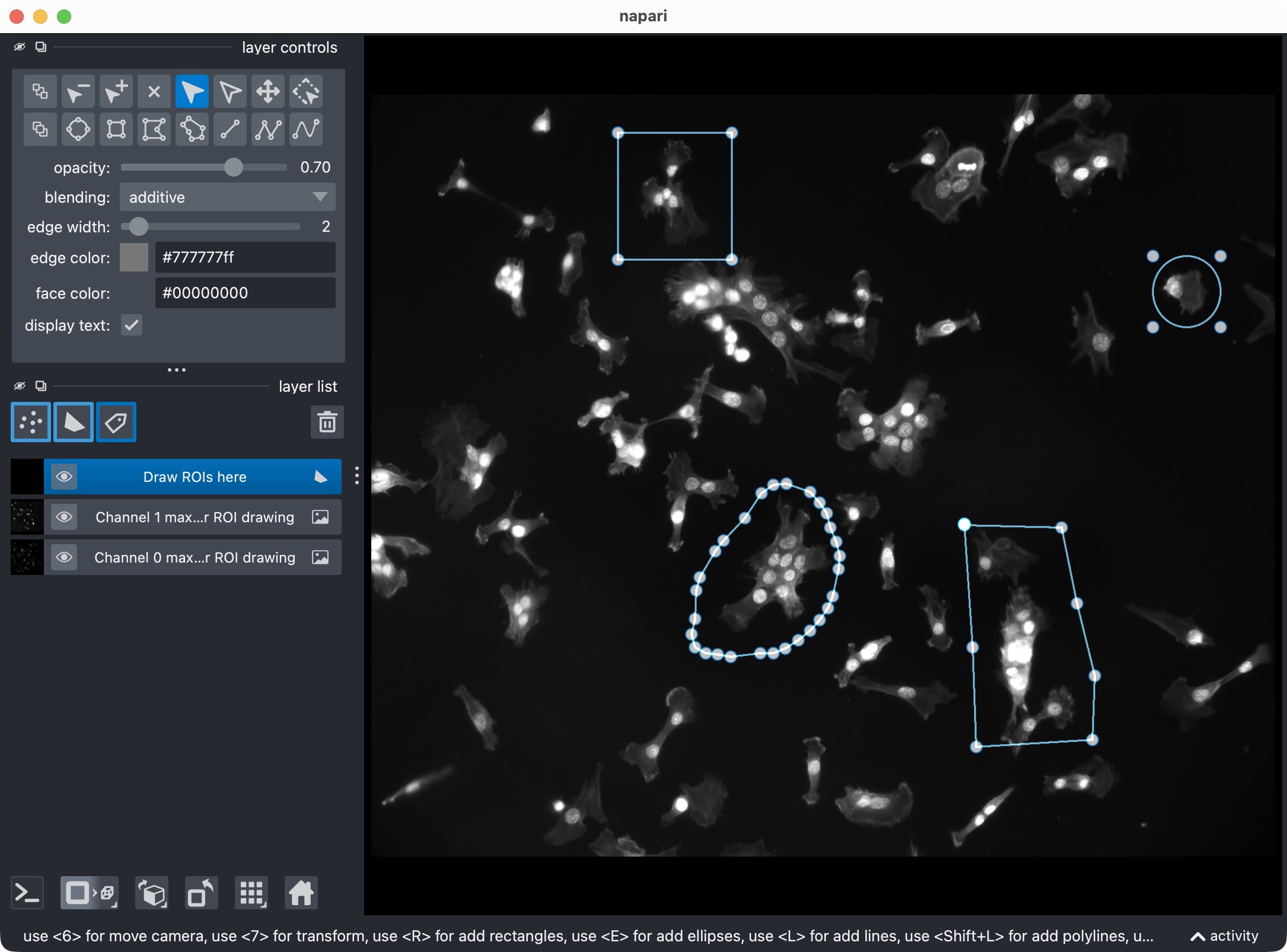
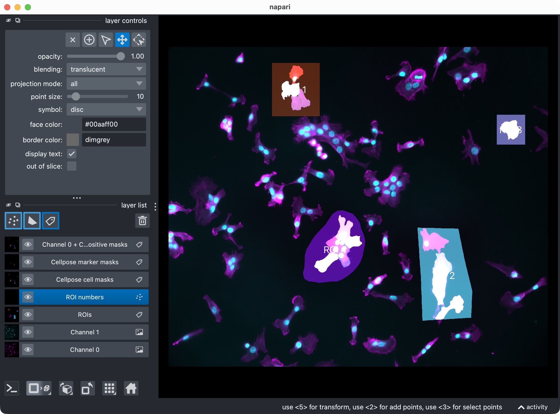
If activated, this is how the ROI drawing step looks in napari. You can draw one or more ROIs with the shapes layer, and then execute the next cell to save the ROIs as a label image for the analysis.

The logic is:

• if USE_FULL_IMAGE_AS_SINGLE_ROI is True, ROI drawing is skipped,

• else, if REUSE_EXISTING_ROI_MASK_IF_AVAILABLE is True, CellColoc first looks for a previously saved ROI label mask in the results directory,

• if such a saved ROI mask exists, it is reused and drawing is skipped,

• if not, napari opens and you can draw one or more ROIs interactively.

This is useful in two common situations:

• first analysis run: you draw the ROIs once,

• later rerun of the same dataset: you reuse the saved ROI mask instead of drawing again.

If you want forced redraw behavior every time, set:

REUSE_EXISTING_ROI_MASK_IF_AVAILABLE = False

Optional: Save drawn ROIs or load an existing ROI mask

The following cell resolves the final ROI mask that will be used for analysis:

if USE_FULL_IMAGE_AS_SINGLE_ROI:
    roi_labels_2d = create_full_image_roi_labels(loaded_images.cell_image.shape[1:])
elif existing_roi_labels is not None:
    roi_labels_2d = existing_roi_labels
elif RUNTIME_CONFIG.draw_rois:
    roi_labels_2d = save_roi_labels_from_shapes(
        shapes_layer=shapes_layer,
        output_path=loaded_images.paths.roi_mask_path,
        image_shape_yx=loaded_images.cell_image.max(axis=0).shape,
        scale_yx=loaded_images.voxel_scale_zyx[1:])
else:
    roi_labels_2d = load_roi_labels(loaded_images.paths.roi_mask_path)

roi_ids = np.unique(roi_labels_2d)
roi_ids = roi_ids[roi_ids != 0]
print(f"ROI ids: {roi_ids}")

This cell supports three modes:

Whole-image mode

If USE_FULL_IMAGE_AS_SINGLE_ROI is True, CellColoc creates one ROI that spans the complete image.

This is the simplest entry point for 2D analysis and the default assumption in this tutorial.

Interactive ROI mode

If whole-image mode is disabled and you drew ROIs in napari, the shapes are rasterized into a label image and saved to the results directory.

Saved ROI reuse mode

If a saved ROI mask was found earlier, that existing label image is loaded and used directly.

After this step, roi_labels_2d contains the actual ROI label map for the analysis, and the script prints the detected ROI IDs.

Run the ROI-wise segmentation and colocalization analysis

This is the main analysis step:

run_result = run_roi_cellpose_colocalization(
    loaded_images           = loaded_images,
    roi_labels_2d           = roi_labels_2d,
    cell_model_config       = CELL_MODEL_CONFIG,
    marker_model_config     = MARKER_MODEL_CONFIG,
    colocalization_config   = COLOCALIZATION_CONFIG,
    runtime_config          = RUNTIME_CONFIG,
    optional_region_result  = None)
# print the first 3 columns of the overview table for a quick check:
print("Overview of the colocalization results (first 3 columns):")
print(run_result.tables.overview.iloc[:, :3])

What happens here:

• each ROI is processed separately,

• the cell channel is segmented according to CELL_MODEL_CONFIG,

• the marker channel is segmented according to MARKER_MODEL_CONFIG,

• overlap between both segmentation results is measured,

• positive and negative cells are classified,

• detailed, summary, and overview tables are assembled.

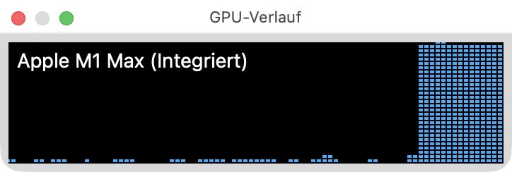
You can cross-check that Cellpose is running on GPU by looking at the console output or the task manager during this step. If you have a compatible GPU and the necessary drivers, you should see messages indicating that Cellpose is using CUDA for segmentation. On macos with Apple Silicon, Cellpose uses the MPS backend, and you should see messages about MPS usage instead.

The function returns a run_result object that contains:

• the full label masks,

• ROI-level and cell-level tables,

• optional Cellpose refinement cache data.

For threshold-based methods this same function would still be used. Only the channel configs would change.

Depending on the size of the image, the number of ROIs, and your computational resources, this step can take a while. If you want to test the workflow on a smaller crop of the image, set:

RUNTIME_CONFIG.crop_for_testing = (slice(0, 1), slice(0, 512), slice(0, 512))

Visualize the result in napari

The next cell opens the current result in napari:

if RUNTIME_CONFIG.open_results:
    viewer = show_analysis_results(
        loaded_images=loaded_images,
        roi_labels_2d=roi_labels_2d,
        run_result=run_result,
        display_names=DISPLAY_NAMES,
        optional_region_result=None)
    print("Inspect the final layers in napari and close the window when finished.")
    napari.run()

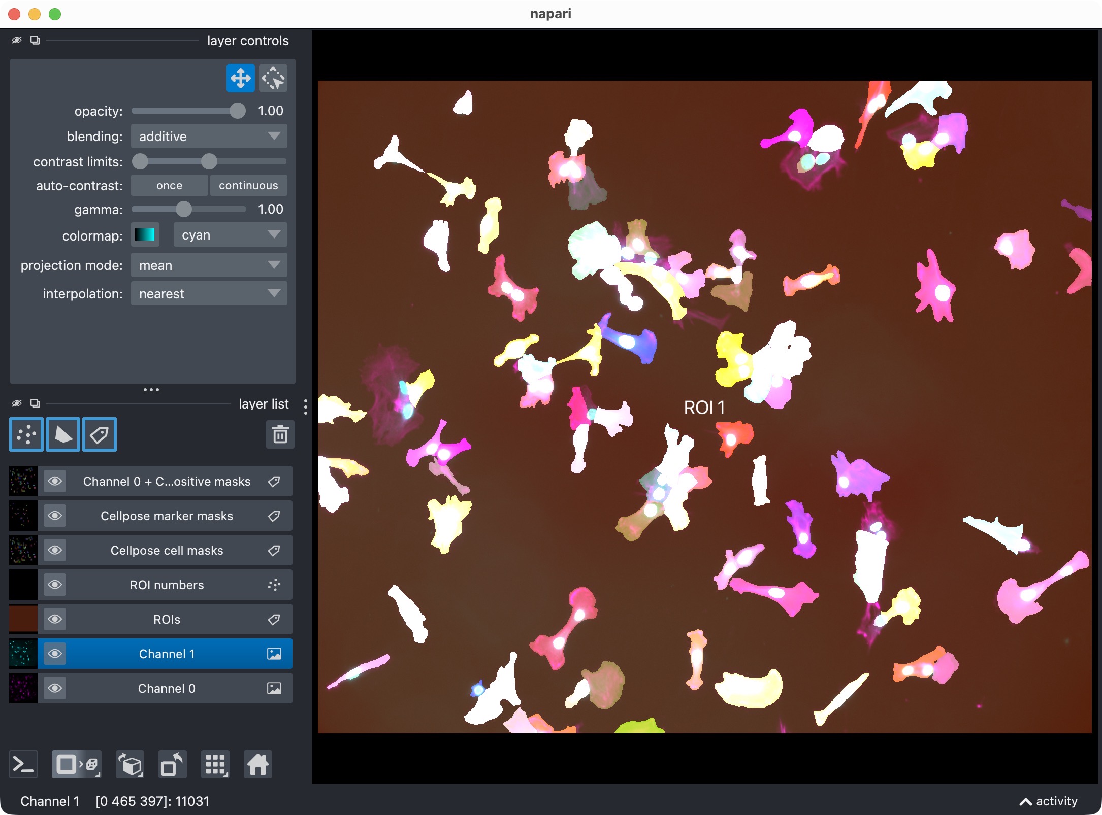
The napari viewer showing the analysis result layers, including the original channels, ROI labels, segmented cell masks, segmented marker masks, and positive-cell mask.

This visualization usually includes:

• the analysis channels,

• the ROI labels,

• the segmented cell masks,

• the segmented marker masks,

• the derived positive-cell mask.

This is the first checkpoint where you inspect whether the segmentation and positivity calls look plausible before refining anything.

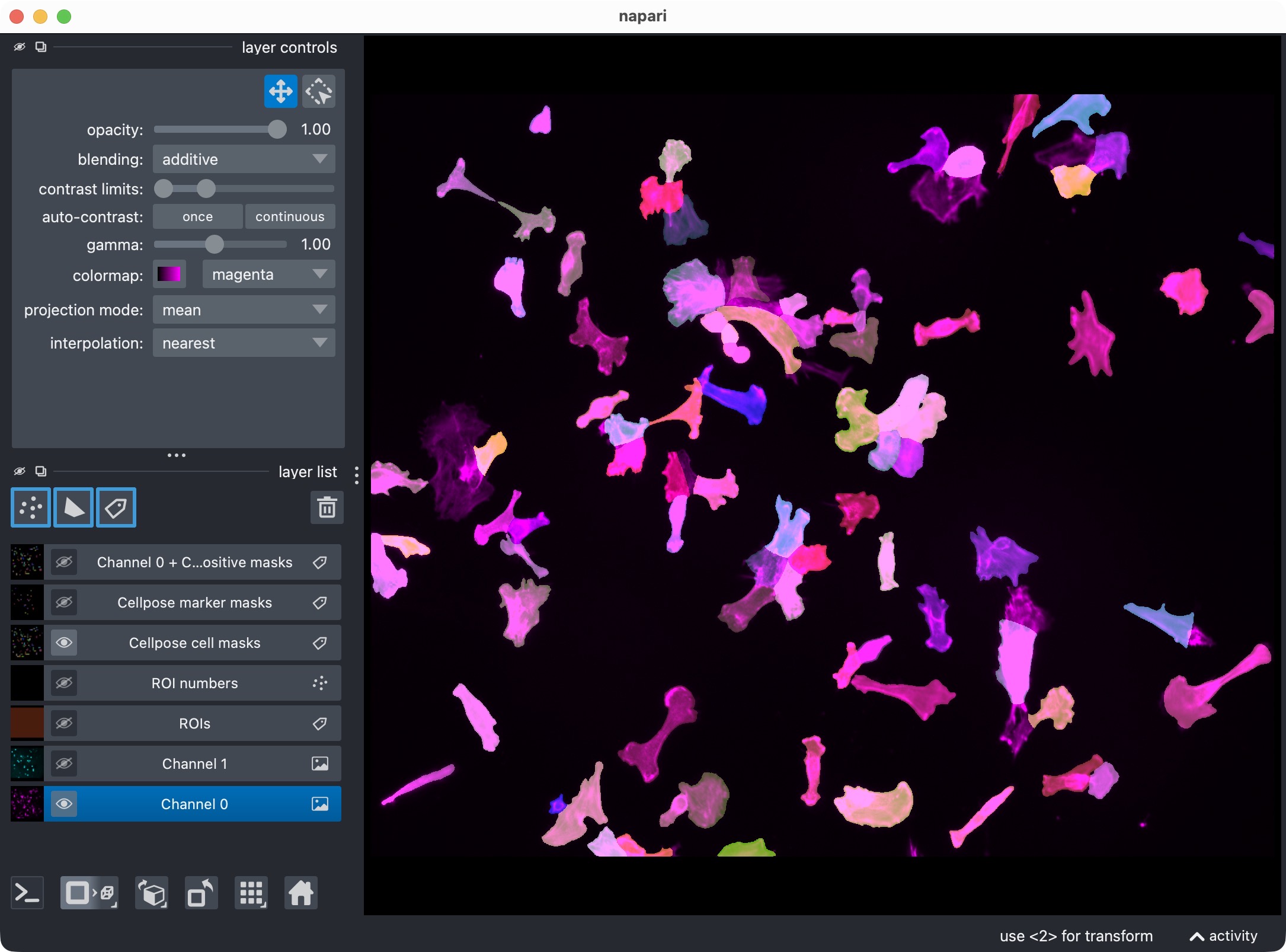
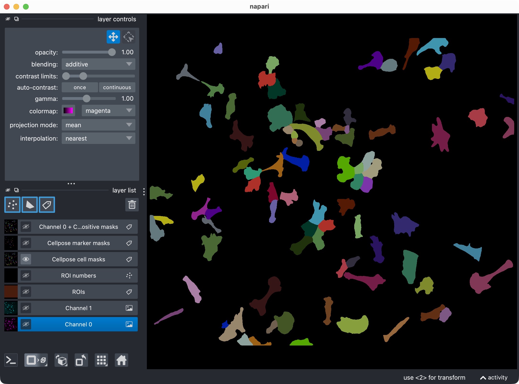
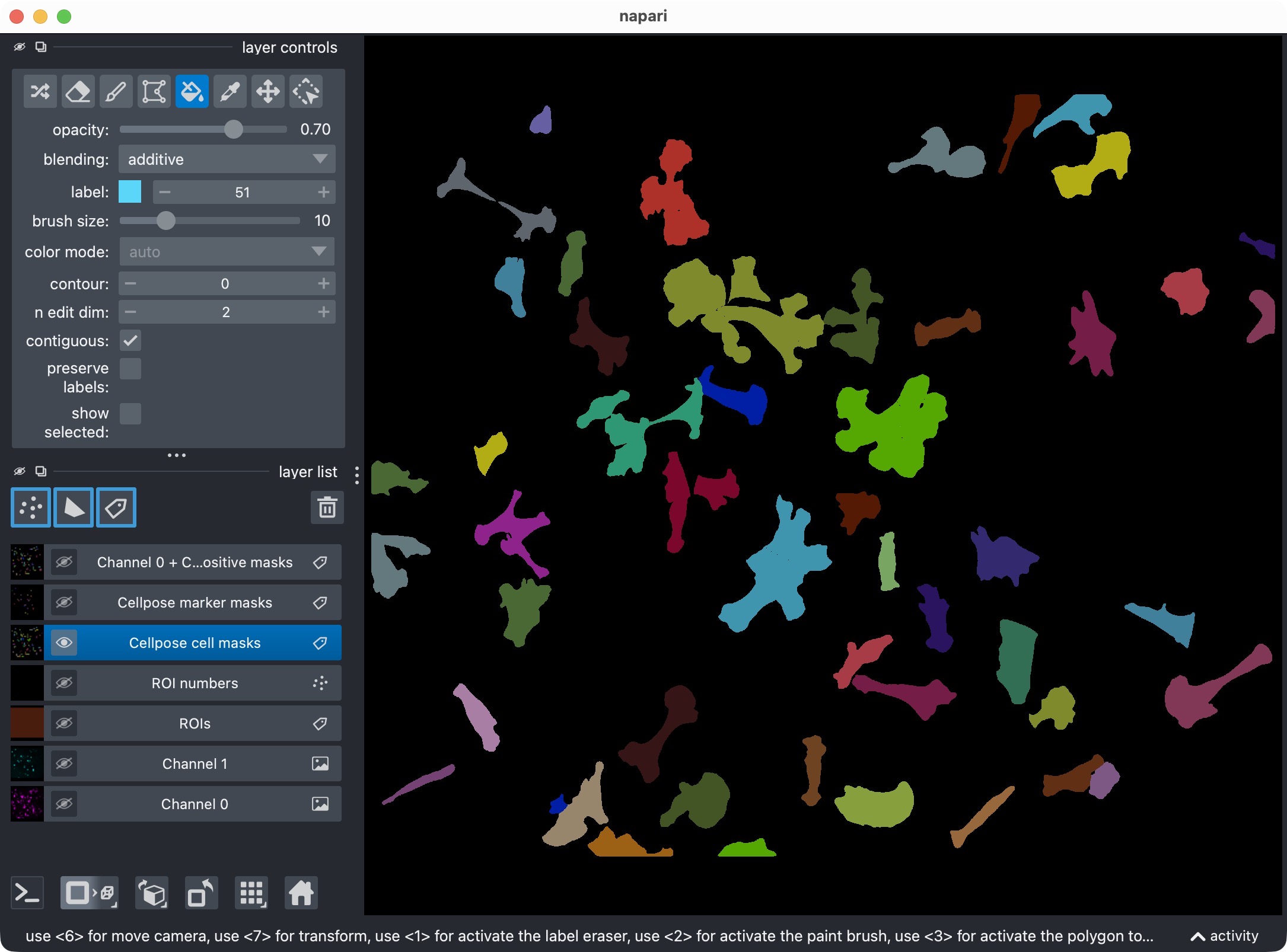
Top: Segmentation result for channel 0 (cell channel) shown in napari together with the original image for reference. Bottom: Segmentation result for channel 0 only, showing the segmented cell masks.

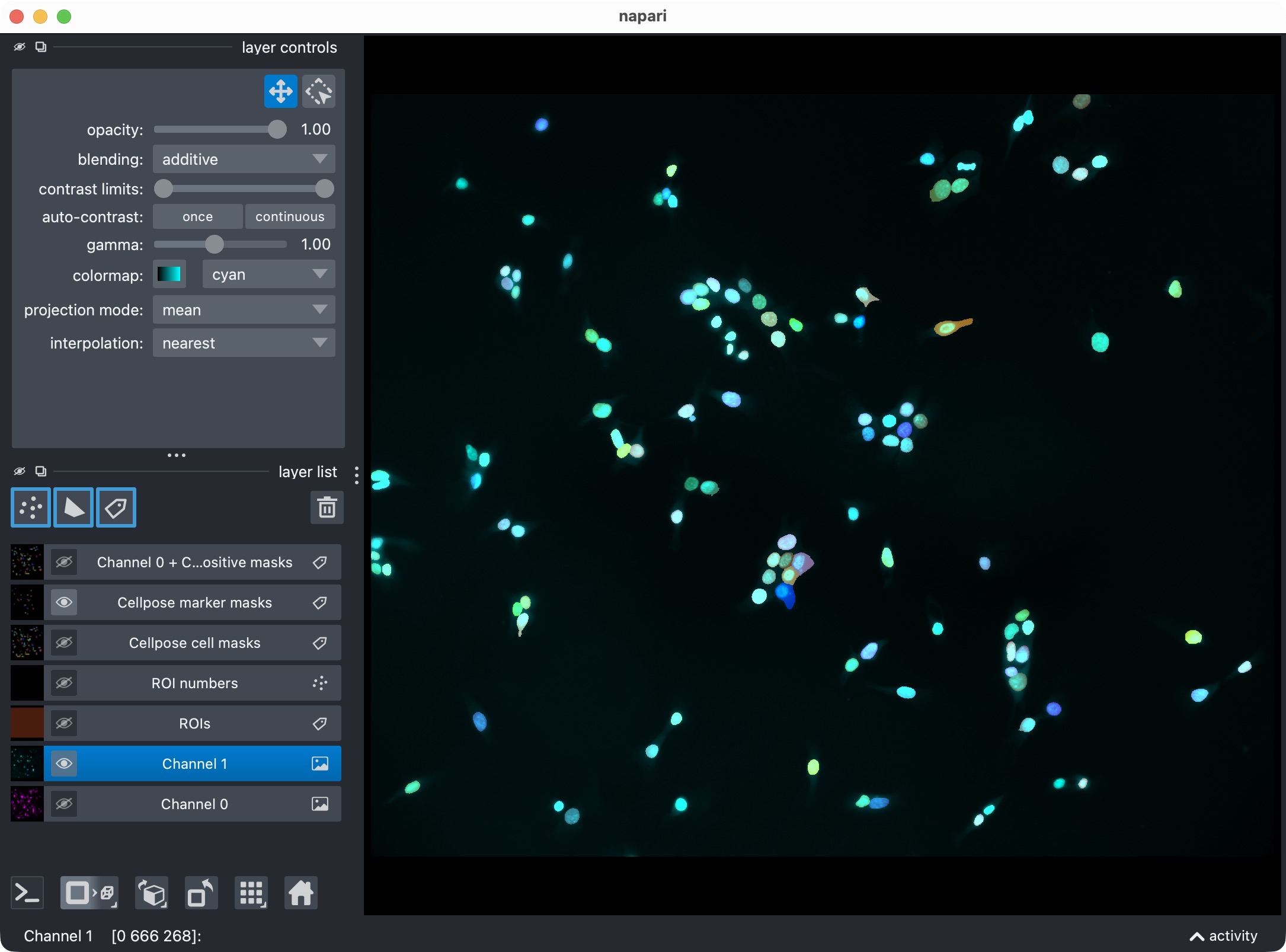
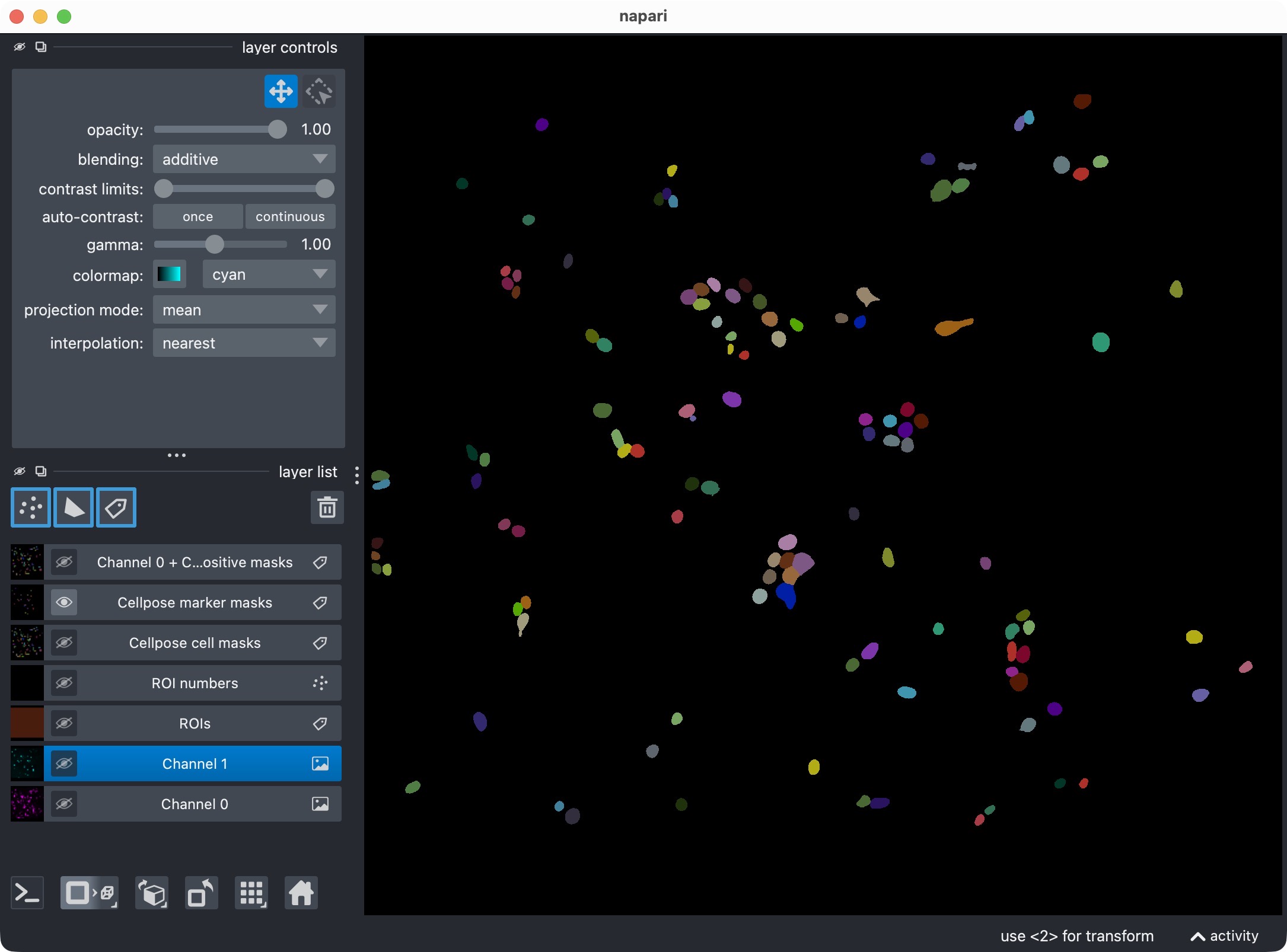
Top: Segmentation result for channel 1 (marker channel) shown in napari together with the original image for reference. Bottom: Segmentation result for channel 1 only, showing the segmented marker masks.

In case you have analyzed individual ROIs instead of the whole image, this is how the ROI labels look in napari. Each ROI is assigned a different integer ID, which enables ROI-wise analysis and result aggregation.

If you want to skip napari output during batch-style testing, set:

RUNTIME_CONFIG.open_results = False

Optional: Refine Cellpose thresholds and inspect the updated result

The next cell performs cache-based post hoc refinement:

REFINE_WITH_CACHED_CELLPOSE_OUTPUTS = True
REFINED_CELL_CELLPROB_THRESHOLD     = CELL_MODEL_CONFIG.cellprob_threshold - 5.0
REFINED_CELL_FLOW_THRESHOLD         = CELL_MODEL_CONFIG.flow_threshold - 0.3
REFINED_MARKER_CELLPROB_THRESHOLD   = MARKER_MODEL_CONFIG.cellprob_threshold
REFINED_MARKER_FLOW_THRESHOLD       = MARKER_MODEL_CONFIG.flow_threshold

if REFINE_WITH_CACHED_CELLPOSE_OUTPUTS:
    run_result = refine_run_result_from_cellpose_cache(
        loaded_images=loaded_images,
        roi_labels_2d=roi_labels_2d,
        run_result=run_result,
        colocalization_config=COLOCALIZATION_CONFIG,
        cell_cellprob_threshold=REFINED_CELL_CELLPROB_THRESHOLD,
        cell_flow_threshold=REFINED_CELL_FLOW_THRESHOLD,
        marker_cellprob_threshold=REFINED_MARKER_CELLPROB_THRESHOLD,
        marker_flow_threshold=REFINED_MARKER_FLOW_THRESHOLD,
        optional_region_result=None)

    print(run_result.tables.overview.iloc[:, :3])

    viewer = show_analysis_results(
        loaded_images=loaded_images,
        roi_labels_2d=roi_labels_2d,
        run_result=run_result,
        display_names=DISPLAY_NAMES,
        optional_region_result=None)
    print("Inspect the refined layers in napari and close the window when finished.")
    napari.run()
else:
    print("Cached Cellpose refinement is disabled for this run.")

This step is useful when the initial Cellpose result is close to correct but slightly too permissive or too conservative.

The refinement works by rebuilding masks from cached Cellpose network outputs instead of rerunning the full network forward pass. This is much faster than running a fresh Cellpose segmentation from scratch.

Relevant refinement settings include:

• REFINE_WITH_CACHED_CELLPOSE_OUTPUTS: enable or disable the refinement step.

• REFINED_CELL_CELLPROB_THRESHOLD and REFINED_CELL_FLOW_THRESHOLD: new thresholds for the cell channel.

• REFINED_MARKER_CELLPROB_THRESHOLD and REFINED_MARKER_FLOW_THRESHOLD: new thresholds for the marker channel.

If you only want to refine one channel, you can keep the other channel’s thresholds unchanged.

Optional: Reanalyze manually edited label layers from napari

The next cell supports a more manual correction workflow:

REANALYZE_EDITED_LABELS_FROM_VIEWER = True

""" 
In the opened Napari viewer, you can manually edit the Cellpose-generated label layers 
(e.g. using the brush, eraser, or other label editing tools) to correct any segmentation 
errors. When you are done, execute this cell to extract the edited masks from the viewer. 
The colocalization analysis will be re-run based on the edited masks, and the updated results 
will be displayed in a new Napari viewer instance.
"""

if REANALYZE_EDITED_LABELS_FROM_VIEWER:
    cell_masks_from_viewer, marker_masks_from_viewer = extract_label_masks_from_viewer(viewer)
    run_result = analyze_existing_masks(
        loaded_images=loaded_images,
        roi_labels_2d=roi_labels_2d,
        cell_masks=cell_masks_from_viewer,
        marker_masks=marker_masks_from_viewer,
        colocalization_config=COLOCALIZATION_CONFIG,
        optional_region_result=None,
        cell_refinement_context=run_result.cell_refinement_context,
        marker_refinement_context=run_result.marker_refinement_context,
    )

    print(run_result.tables.overview.iloc[:, :3])

    viewer = show_analysis_results(
        loaded_images=loaded_images,
        roi_labels_2d=roi_labels_2d,
        run_result=run_result,
        display_names=DISPLAY_NAMES,
        optional_region_result=None,
    )
    print("Inspect the relabeled result in napari and close the window when finished.")
    napari.run()
else:
    print("Manual label reanalysis from the napari viewer is disabled for this run.")

Manually edited label layers in napari. In this example, the user has manually edited the marker mask layer to correct a segmentation error. After running the current cell, the updated masks will be reanalyzed and the results will be updated accordingly.

This is useful when:

• Cellpose split one object into several labels,

• Cellpose missed a merge or introduced a false positive,

• you want to manually correct the label layers directly in napari.

The workflow is:

1. inspect the result in napari,

2. edit the label layers manually,

3. run this cell,

4. let CellColoc recompute the tables from the updated masks.

The underlying image data are not resegmented here. Instead, the edited mask layers are read back from napari and analyzed as the new truth for this run.

Export results

The final cell writes the outputs to disk:

export_analysis_outputs(
    run_result=run_result,
    paths=loaded_images.paths,
    optional_region_result=None)
print("Final results exported.")

The exported results are written to the dataset’s results/ directory.

Typical outputs include:

• ROI mask,

• cell mask,

• marker mask,

• positive-cell mask,

• detailed CSV tables,

• a combined Excel workbook with the overview, summary, and detailed tables.

The export is intentionally placed at the end of the interactive workflow so that the saved outputs reflect the final accepted analysis state rather than an early intermediate result.

Understanding the exported Excel workbook

In addition to the CSV export, CellColoc writes one Excel workbook.

For this two-channel colocalization workflow, the three central colocalization-oriented worksheets are:

• detailed_overlaps: one row per concrete cell-marker overlap event. This is the most granular table and is useful if you want to inspect exactly which cell object overlapped which marker object and by how much.

• cell_summary: one row per segmented cell. This table aggregates overlap events to the cell level and contains the final positive or negative classification of each cell.

• roi_coloc_overview: one row per ROI. This table summarizes the analysis at the region level and is usually the best starting point for comparing different ROIs or different files at a glance.

In the current CellColoc release, the workbook may additionally contain further sheets with morphology and per-ROI summary metrics, for example channel-specific object-property tables. Those tables are described in more detail on the dedicated results reference page:

usage_results.html

In this tutorial, we focus only on the core object-based colocalization outputs.

For many downstream analyses, roi_coloc_overview is the most compact result table because it combines ROI geometry, object counts, positivity counts, and occupancy metrics in one place.

Understanding the roi_coloc_overview columns

The exact set of columns depends on whether you analyze only the two primary channels or also an optional third analysis channel. The groups below explain the meaning of the standard columns.

ROI identity and object counts

• roi_id: integer ID of the ROI in the ROI label image.

• n_cells: number of segmented cell objects inside the ROI.

• n_marker_positive_cells: number of cells in that ROI that satisfy the configured marker-positivity rule.

• n_marker_objects: number of segmented marker objects inside the ROI.

If an optional third analysis channel is configured with additional cell-positivity evaluation, the following columns may also appear:

• n_optional_region_positive_cells: number of cells that are positive with respect to the optional third channel.

• n_marker_and_optional_region_positive_cells: number of double-positive cells, that is, cells that are positive for both the main marker channel and the optional third channel.

ROI geometry

• drawn_roi_area_px: 2D ROI area in pixels.

• drawn_roi_area_um2: 2D ROI area converted to square micrometers using VOXEL_SCALE_ZYX.

• roi_volume_voxels: analysis ROI volume in voxels. In a pure 2D workflow this is effectively the ROI area multiplied by the analyzed z-depth, which is usually one plane.

• roi_volume_um3: physical ROI volume in cubic micrometers.

These geometry values are the denominators for the occupancy metrics described below.

Cell-channel occupancy

These columns quantify how much of the ROI is occupied by the segmented cell channel:

• cell_occupancy_area_px_2d_projection

• cell_occupancy_area_um2_2d_projection

• cell_occupancy_coverage_2d_percent

• cell_occupancy_volume_voxels_3d

• cell_occupancy_volume_um3_3d

• cell_occupancy_coverage_3d_percent

Interpretation:

• the *_2d_projection columns describe the occupied area after projecting the segmented channel along z,

• the *_3d columns describe the occupied voxel volume in the analyzed stack.

For true 2D datasets, the volumetric values are still reported for consistency, but they effectively correspond to a single analyzed z-plane.

Marker-channel occupancy

The same metric family is reported for the segmented marker channel:

• marker_occupancy_area_px_2d_projection

• marker_occupancy_area_um2_2d_projection

• marker_occupancy_coverage_2d_percent

• marker_occupancy_volume_voxels_3d

• marker_occupancy_volume_um3_3d

• marker_occupancy_coverage_3d_percent

These columns are especially helpful when you want to compare how strongly the marker channel fills each ROI independently of the object-based positivity classification.

Optional third-channel occupancy

If an optional third analysis channel is enabled, a third block of occupancy columns is added with the prefix optional_region_:

• optional_region_occupancy_area_px_2d_projection

• optional_region_occupancy_area_um2_2d_projection

• optional_region_occupancy_coverage_2d_percent

• optional_region_occupancy_volume_voxels_3d

• optional_region_occupancy_volume_um3_3d

• optional_region_occupancy_coverage_3d_percent

These columns are useful for lesion coverage, infiltration coverage, tissue occupancy, or any other third-channel segmentation that should be summarized at the ROI level.

How to read the table in practice

As a simple reading strategy:

1. start with roi_id to identify the ROI,

2. check n_cells and n_marker_positive_cells to understand the object counts,

3. use drawn_roi_area_* and roi_volume_* to understand the ROI size,

4. compare the different *_occupancy_* blocks to quantify how strongly each segmented channel fills the ROI.

This makes roi_coloc_overview the most useful sheet for quick ROI-level quality control and for compact downstream statistics.

Adapting this tutorial to your own data

To reuse this workflow for your own 2D microscopy project, the most important places to adapt are:

• DATA_PATH

• CHANNEL_CONFIG

• DISPLAY_NAMES

• VOXEL_SCALE_ZYX or automatic metadata-based scaling

• CELL_MODEL_CONFIG

• MARKER_MODEL_CONFIG

• COLOCALIZATION_CONFIG

• USE_FULL_IMAGE_AS_SINGLE_ROI and REUSE_EXISTING_ROI_MASK_IF_AVAILABLE

For a first pass on a new 2D dataset, a very practical strategy is:

1. start with whole-image mode,

2. verify that the segmentation backend and thresholds are reasonable,

3. switch to ROI mode only if you need spatial restriction,

4. use cache-based refinement for final tuning,

5. export only after the result looks correct in napari.