Three-channel analysis with z-projection tutorial
This tutorial walks through a three-channel CellColoc workflow based on the interactive Jupyter notebook
user_scripts/nb_microglia_3D_three_channel_zproject_user_script.ipynb,
which is identical to the interactive Python script
user_scripts/microglia_3D_three_channel_zproject_user_script.py.
The goal of this tutorial is to show when and how a nominally 3D microscopy stack can be projected along the z axis before segmentation and downstream colocalization analysis. This can be a very useful strategy because true 3D Cellpose segmentation is computationally expensive.
When, and only when,
the *same* biological cells are visible in the relevant channels,
these channels mainly differ in staining or marker identity rather than in which objects are present,
and the cells are not densely stacked on top of one another along z,
then a z-projection can be a good approximation.
In that situation, CellColoc’s z-projection workflow often offers two practical advantages:
the analysis becomes substantially faster,
and the projected 2D image may even segment more robustly because signal from many z slices is compressed into one plane.
But this comes with a tradeoff: By projecting, you deliberately give up one spatial axis and therefore lose true 3D object geometry. This tutorial therefore shows z-projection as an optional strategy and not as a universal replacement for full 3D analysis.
Dataset used in this tutorial
The tutorial uses the microglia example data set distributed with CellColoc in
example_data/microglia_3D/
Please download the example data from the CellColoc Zenodo example-data record first, as described in the Example data set section. Store the downloaded files locally in a convenient place. For the remainder of this tutorial, we assume that the downloaded files are available relative to the current working directory or current example script in:
example_data/microglia_3D/
The script is written to handle one selected file from that folder at a time.
This is a real 3D multichannel fluorescence dataset. In this tutorial, we treat:
channel 0 as the primary
cellchannel (Cx3cr1-tdTomatomicroglia reporter signal),channel 1 as the first marker channel (
Iba1staining),channel 2 as the optional third analysis channel (
DAPIin this demo setup).
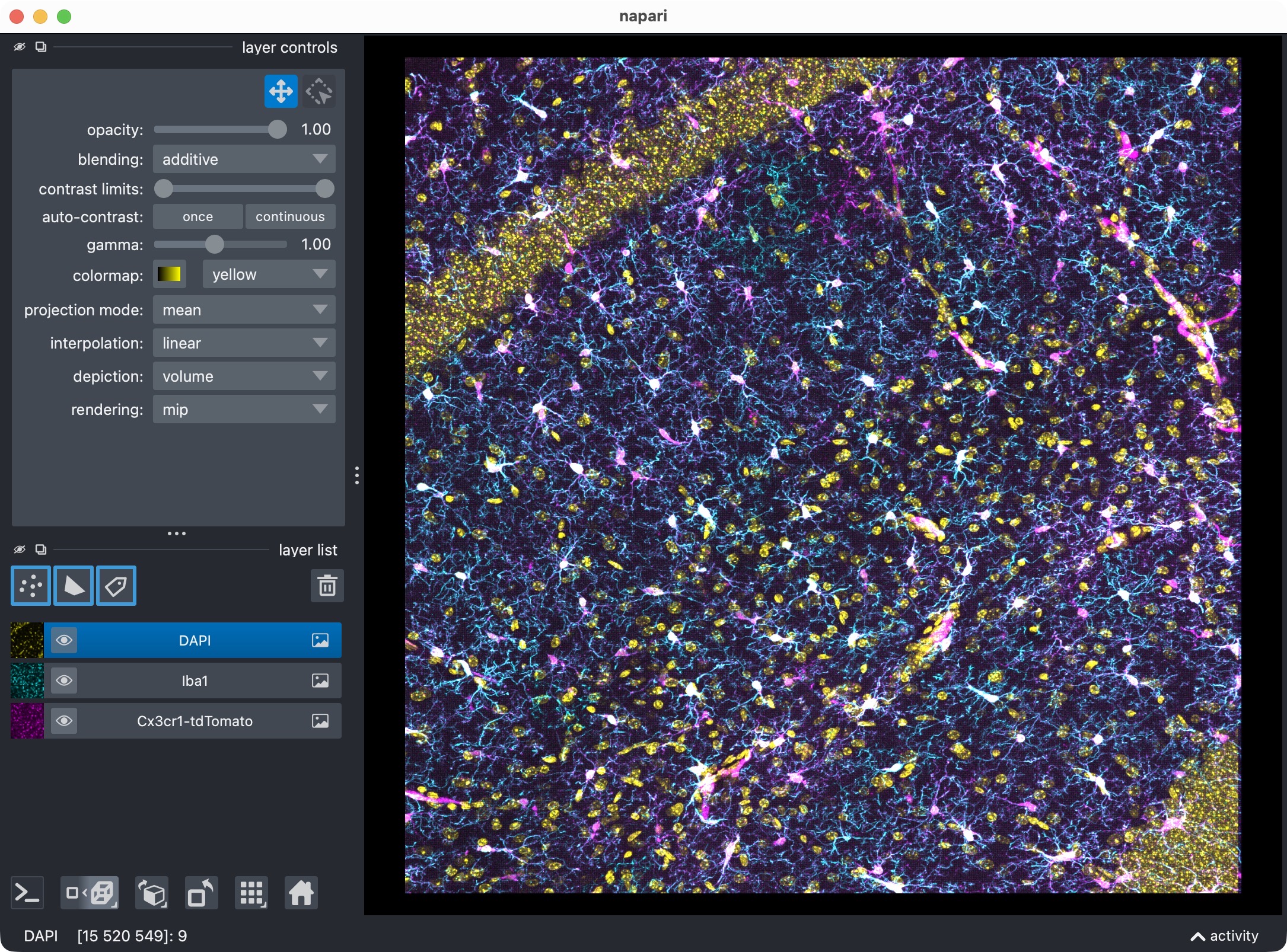
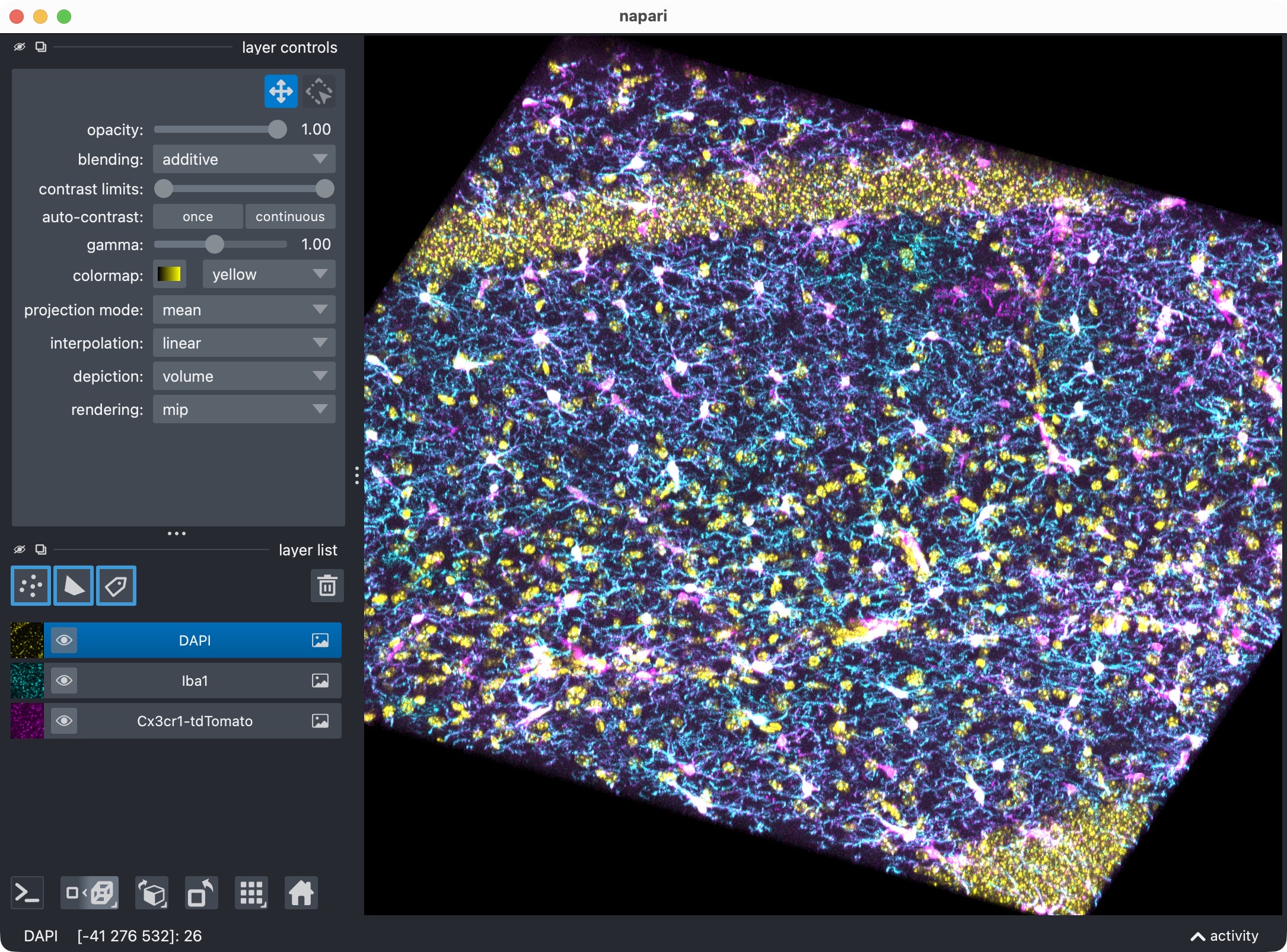
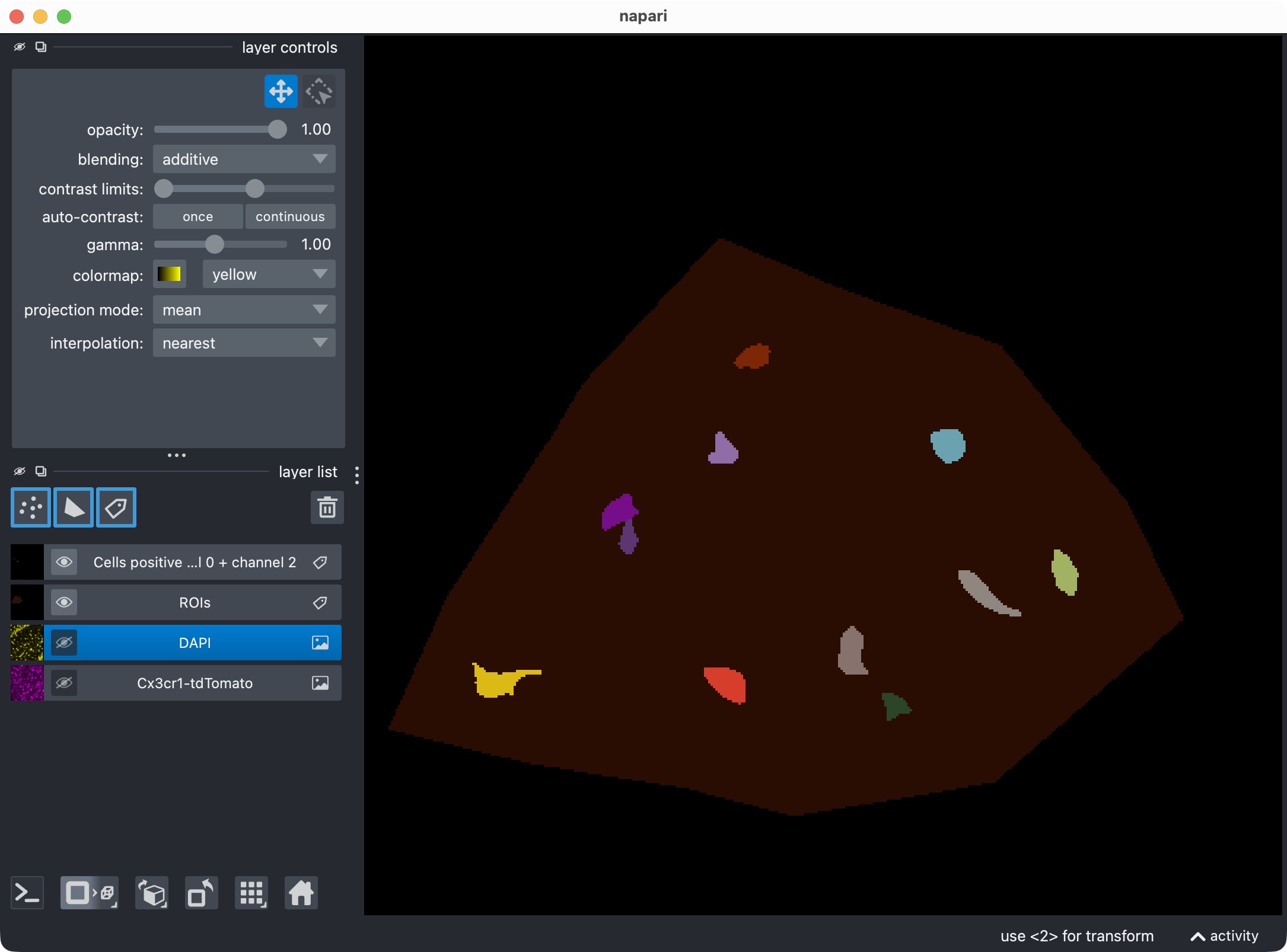
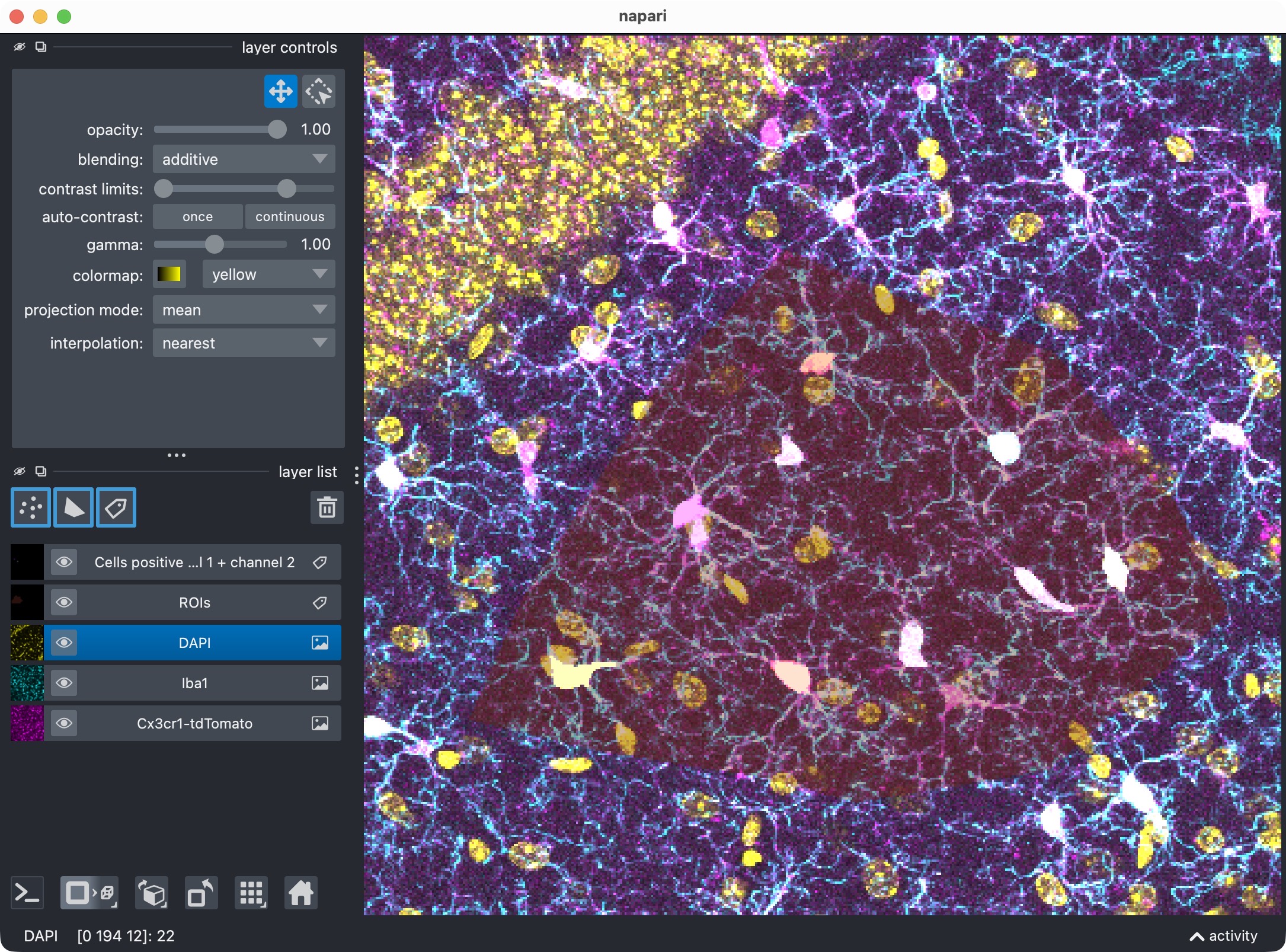
The 3D multi-channel image stack with the raw microglia (magenta), Iba1 (cyan), and DAPI (yellow) channels shown in Napari. Top shows 2D representation, bottom shows 3D representation. The DAPI channel is used for anatomical orientation but not segmented in this tutorial. The microglia channel is segmented with Cellpose, while the Iba1 channel is segmented with Otsu thresholding.
The biological idea of this tutorial is to demonstrate the mechanics of:
projecting a 3D stack into a 2D analysis view,
segmenting multiple channels on that projected view,
evaluating channel-0 positivity against both channel 1 and channel 2,
and inspecting the resulting positivity combinations separately.
How to use this tutorial
The associated user script
user_scripts/nb_microglia_3D_three_channel_zproject_user_script.ipynb
is organized in cells, reflecting the structure of this tutorial. The same
applies to the alternative Python script (there: # %% cells)
user_scripts/microglia_3D_three_channel_zproject_user_script.py.
The recommended way to follow this tutorial is:
open
user_scripts/nb_microglia_3D_three_channel_zproject_user_script.ipynboruser_scripts/microglia_3D_three_channel_zproject_user_script.py,run the cells from top to bottom,
adapt the configuration values for your own dataset only where needed.
The subsections below follow the same order as the script cells.
Imports
The first cell imports the public CellColoc API, napari, NumPy, and
dataclasses.replace:
from pathlib import Path
from dataclasses import replace

import napari
import numpy as np

from cellcoloc import (
    CellposeModelConfig,
    ChannelConfig,
    ColocalizationConfig,
    DisplayNames,
    RuntimeConfig,
    analyze_existing_masks,
    build_positive_cell_mask,
    create_full_image_roi_labels,
    create_roi_drawing_viewer,
    export_analysis_outputs,
    extract_label_masks_from_viewer,
    load_analysis_images,
    load_roi_labels,
    prepare_loaded_images_for_analysis,
    refine_run_result_from_cellpose_cache,
    run_roi_cellpose_colocalization,
    save_roi_labels_from_shapes,
    show_analysis_results,
    try_load_roi_labels)

PROJECT_ROOT = Path(__file__).resolve().parents[1]
What this cell does:
locates the repository root,
imports the reusable CellColoc workflow functions,
imports napari for ROI drawing and interactive inspection,
imports
build_positive_cell_maskfor the dedicated positivity views at the end,imports
replaceso that temporary refinement configs can be derived from the original base configs without overwriting them.
Project settings
The project settings cell contains the full configuration for this projected three-channel workflow:
DATA_DIR = PROJECT_ROOT / "example_data" / "microglia_3D"
DATA_PATHS = sorted(DATA_DIR.glob("*"))
allowed_extensions = [".czi", ".tif", ".tiff", ".ome.tif", ".ome.tiff"]
DATA_PATHS = [p for p in DATA_PATHS if p.suffix.lower() in allowed_extensions]
DATA_PATHS = [p for p in DATA_PATHS if not p.name.startswith(".")]

CHANNEL_CONFIG = ChannelConfig(
    cell_channel=0,
    marker_channel=1,
    optional_region_channel=2)

DISPLAY_NAMES = DisplayNames(
    cell="Cx3cr1-tdTomato",
    marker="Iba1",
    optional_region="DAPI",
    positive_cells="tdTomato + Iba1 positive masks")

VOXEL_SCALE_ZYX = None

CELL_MODEL_CONFIG = CellposeModelConfig(
    model_name_or_path="cpsam",
    segmentation_method="cellpose",
    diameter=None,
    z_crop=None,        # None; optional global analysis z crop as (start, stop); applies to all channels and all ROIs
    z_projection="max",  # None, "max", "mean", "median", "std", or "var"
    anisotropy=True,
    flow3d_smooth=0,
    prefilter=None,
    prefilter_sigma_xy=0.0,
    prefilter_sigma_z=0.0,
    prefilter_median_size_xy=3,
    prefilter_median_size_z=3,
    postfilters=None,
    min_intensity_measure="mean",
    min_intensity_threshold=None,
    local_contrast_k=1.0,
    local_contrast_shell_inner_radius=1,
    local_contrast_shell_outer_radius=4,
    bright_pixel_measure="count",
    bright_pixel_threshold=None,
    bright_pixel_min_count=None,
    bright_pixel_min_fraction=None,
    cellprob_threshold=1.5,
    flow_threshold=0.4)

MARKER_MODEL_CONFIG = CellposeModelConfig(
    model_name_or_path="cpsam",
    segmentation_method="otsu",
    diameter=None,
    # z_crop=None,
    # z_projection="max", # it's not necessary to repeat z-projection option in marker channel; when set in the cell channel, it will be applied to all channels
    anisotropy=True,
    flow3d_smooth=0,
    prefilter=None,
    prefilter_sigma_xy=0.0,
    prefilter_sigma_z=0.0,
    prefilter_median_size_xy=3,
    prefilter_median_size_z=3,
    postfilters=None,
    min_intensity_measure="mean",
    min_intensity_threshold=None,
    local_contrast_k=1.0,
    local_contrast_shell_inner_radius=1,
    local_contrast_shell_outer_radius=4,
    bright_pixel_measure="count",
    bright_pixel_threshold=None,
    bright_pixel_min_count=None,
    bright_pixel_min_fraction=None,
    cellprob_threshold=0.0,
    flow_threshold=0.4)

OPTIONAL_REGION_MODEL_CONFIG = CellposeModelConfig(
    model_name_or_path="cpsam",
    segmentation_method="cellpose",
    diameter=None,
    #z_crop=None,
    #z_projection="max", # it's not necessary to repeat z-projection option in optional region channel; when set in the cell channel, it will be applied to all channels
    anisotropy=True,
    flow3d_smooth=0,
    prefilter=None,
    prefilter_sigma_xy=0.0,
    prefilter_sigma_z=0.0,
    prefilter_median_size_xy=3,
    prefilter_median_size_z=3,
    postfilters=None,
    min_intensity_measure="mean",
    min_intensity_threshold=None,
    local_contrast_k=1.0,
    local_contrast_shell_inner_radius=1,
    local_contrast_shell_outer_radius=4,
    bright_pixel_measure="count",
    bright_pixel_threshold=None,
    bright_pixel_min_count=None,
    bright_pixel_min_fraction=None,
    cellprob_threshold=0.0,
    flow_threshold=0.4)

"""
To exclude the optional third channel from segmentation and from the downstream
cell-positivity analysis, update the script as follows:

1. In ``CHANNEL_CONFIG``, set:

   ``optional_region_channel=None``

2. Set this variable to:

   ``OPTIONAL_REGION_MODEL_CONFIG = None``

3. In ``COLOCALIZATION_CONFIG``, set:

   ``evaluate_optional_region_cell_positivity=False``

4. Skip or remove the later visualization cells that explicitly show:

   - channel 0 + channel 2 positive cells
   - channel 0 + channel 1 + channel 2 positive cells

This reduces the workflow back to an ordinary two-channel analysis while
keeping the rest of the script structure intact.
"""

COLOCALIZATION_CONFIG = ColocalizationConfig(
    min_cell_voxels=50,
    overlap_fraction_threshold=0.02,
    min_overlap_voxels=10,
    evaluate_optional_region_cell_positivity=True)

RUNTIME_CONFIG = RuntimeConfig(
    draw_rois=True,
    process_rois=True,
    open_results=True,
    use_gpu=True,
    crop_for_testing=None,
    image_loading_mode="memap")

USE_FULL_IMAGE_AS_SINGLE_ROI = False
REUSE_EXISTING_ROI_MASK_IF_AVAILABLE = True
INITIAL_RESULT_LAYER_KEYS = [
    "cell_image",
    "marker_image",
    "optional_region_image",
    "rois",
    "roi_numbers",
    "cell_masks",
    "marker_masks",
    "positive_cells",
    "optional_region_labels"]
REFINEMENT_RESULT_LAYER_KEYS = [
    "cell_masks",
    "marker_masks",
    "positive_cells",
    "optional_region_labels",
    "rois"]

print("Detected input files:")
for data_path in DATA_PATHS:
    print(f" - {data_path.name}")

SELECTED_FILE_NAME = DATA_PATHS[0].name
DATA_PATH = DATA_DIR / SELECTED_FILE_NAME
print(f"Selected file for analysis:\n{DATA_PATH}")
This is the most important cell to adapt for your own projected 3D analysis.
Input-file discovery and selection
The script scans example_data/microglia_3D/ for supported microscopy files
and lets you select one through:
SELECTED_FILE_NAME = DATA_PATHS[0].name
To analyze a different stack from the same folder, simply change that assignment.
Channel assignment and display names
CHANNEL_CONFIG assigns the three analysis channels:
cell_channel=0marker_channel=1optional_region_channel=2
DISPLAY_NAMES controls how those channels and result layers appear in
napari.
In this tutorial, all three channels are part of the analysis. The third channel is not only displayed for orientation, but also segmented and included in downstream per-cell positivity analysis.
Voxel scale
VOXEL_SCALE_ZYX is set to None here. This tells CellColoc to first try
to resolve the voxel size from OMIO metadata. If needed, you can also provide
it explicitly as:
a full
(Z, Y, X)tuple for 3D datasets,or, for 2D-oriented workflows, as a shorter
(Y, X)tuple.
Why z-projection is configured in the cell config
The key option for this tutorial is:
z_projection="max"
in CELL_MODEL_CONFIG.
This tells CellColoc to project the stack along z before segmentation and analysis. Supported projection methods are:
None: do not project,"max""mean""median""std""var"
If you additionally define z_crop=(z_start, z_stop), only that z interval
is projected.
Once a projection is active:
CellColoc automatically applies the same projection to all channels,
the analysis runs on the resulting 2D view rather than on the full 3D stack,
later visualizations also show the projected analysis image,
and Cellpose is automatically run in the effective 2D mode for the projected channel.
Segmentation configurations
This tutorial defines three channel configs:
CELL_MODEL_CONFIGMARKER_MODEL_CONFIGOPTIONAL_REGION_MODEL_CONFIG
The important idea is that CellColoc lets you mix segmentation backends even in a projected workflow.
In the current script:
channel 0 uses Cellpose with
segmentation_method="cellpose",channel 1 uses a classical threshold-based workflow with
segmentation_method="otsu",channel 2 uses Cellpose again.
This mixed setup is deliberate. It shows that z-projection is not tied to one single segmentation backend.
Optional third channel
OPTIONAL_REGION_MODEL_CONFIG activates segmentation of the third channel.
Directly below that config, the script contains an explanatory block showing
how to disable the third channel again if you want to fall back to a
two-channel workflow.
In short, you would then:
set
optional_region_channel=NoneinCHANNEL_CONFIG,set
OPTIONAL_REGION_MODEL_CONFIG = None,set
evaluate_optional_region_cell_positivity=FalseinCOLOCALIZATION_CONFIG,and skip the later dedicated third-channel positivity views.
Third-channel positivity evaluation
The key switch that activates per-cell positivity analysis against channel 2 is:
evaluate_optional_region_cell_positivity=True
inside COLOCALIZATION_CONFIG.
This means the script reports not only:
which channel-0 cells are positive against channel 1,
but also:
which channel-0 cells are positive against channel 2,
and which channel-0 cells are positive for both channel 1 and channel 2.
Runtime settings and ROI mode
The runtime settings control the interactive analysis mode:
image_loading_mode="memap"uses OMIO’s disk-backed loading mode,USE_FULL_IMAGE_AS_SINGLE_ROI = Falseenables ROI-based analysis,REUSE_EXISTING_ROI_MASK_IF_AVAILABLE = Truereuses a saved ROI mask when available.
If you want to analyze the full field of view as one ROI, set:
USE_FULL_IMAGE_AS_SINGLE_ROI = True
Load the analysis channels
The next cell loads the selected stack and then prepares the projected analysis view:
loaded_images = load_analysis_images(
    source_path=DATA_PATH,
    channel_config=CHANNEL_CONFIG,
    voxel_scale_zyx=VOXEL_SCALE_ZYX,
    crop_for_testing=RUNTIME_CONFIG.crop_for_testing,
    image_loading_mode=RUNTIME_CONFIG.image_loading_mode)
loaded_images = prepare_loaded_images_for_analysis(
    loaded_images,
    CELL_MODEL_CONFIG,
    MARKER_MODEL_CONFIG,
    OPTIONAL_REGION_MODEL_CONFIG)
print(f"Results directory:\n{loaded_images.paths.results_dir}")
print("Prepared analysis view: "
      f"shape={loaded_images.cell_image.shape}, "
      f"is_3d={loaded_images.is_3d}, "
      f"z_projection={loaded_images.z_projection_method!r}, "
      f"analysis_z_bounds={loaded_images.analysis_z_bounds}")

existing_roi_labels = None
if REUSE_EXISTING_ROI_MASK_IF_AVAILABLE:
    existing_roi_labels = try_load_roi_labels(loaded_images.paths.roi_mask_path)
This is the key difference from the standard full-3D workflow.
The sequence is:
load the original microscopy stack through OMIO,
extract the configured channels,
call
prepare_loaded_images_for_analysis(...),obtain the projected 2D analysis image that will be used by all later steps.
The printed status output tells you:
the prepared image shape,
whether the resulting analysis view is effectively 3D or not,
which z-projection method was applied,
and which z interval was used.
Draw ROIs interactively in napari
The ROI-drawing cell behaves just like in the other tutorials:
if USE_FULL_IMAGE_AS_SINGLE_ROI:
    print("Whole-image mode is enabled. ROI drawing is skipped.")
elif existing_roi_labels is not None:
    print("An existing ROI mask was found and will be reused. ROI drawing is skipped.")
elif RUNTIME_CONFIG.draw_rois:
    roi_viewer, shapes_layer = create_roi_drawing_viewer(
        loaded_images=loaded_images,
        display_names=DISPLAY_NAMES,
    )
    print("Draw ROIs in napari and close the window. Then run the next cell.")
    napari.run()
else:
    print("ROI drawing is disabled. The next cell will load an existing ROI mask from disk.")
Because the analysis image has already been projected, the ROI drawing now happens on the projected 2D view rather than on the original 3D stack.
This is exactly what you want in a projected workflow: the ROIs should match the image that will actually be segmented and analyzed.
Save the drawn ROIs or load an existing ROI mask
The next cell resolves the ROI source:
if USE_FULL_IMAGE_AS_SINGLE_ROI:
    roi_labels_2d = create_full_image_roi_labels(loaded_images.cell_image.shape[1:])
elif existing_roi_labels is not None:
    roi_labels_2d = existing_roi_labels
elif RUNTIME_CONFIG.draw_rois:
    roi_labels_2d = save_roi_labels_from_shapes(
        shapes_layer=shapes_layer,
        output_path=loaded_images.paths.roi_mask_path,
        image_shape_yx=loaded_images.cell_image.max(axis=0).shape,
        scale_yx=loaded_images.voxel_scale_zyx[1:])
else:
    roi_labels_2d = load_roi_labels(loaded_images.paths.roi_mask_path)

roi_ids = np.unique(roi_labels_2d)
roi_ids = roi_ids[roi_ids != 0]
print(f"ROI ids: {roi_ids}")
result_viewer = None
The order is:
full-image mode if enabled,
otherwise reuse an existing ROI mask when available,
otherwise save the newly drawn ROIs,
otherwise load a previously saved ROI mask explicitly.
The resulting roi_labels_2d is then used for the entire rest of the run.
Run the ROI-wise three-channel segmentation and colocalization analysis
The main analysis cell runs segmentation and table generation:
run_result = run_roi_cellpose_colocalization(
    loaded_images=loaded_images,
    roi_labels_2d=roi_labels_2d,
    cell_model_config=CELL_MODEL_CONFIG,
    marker_model_config=MARKER_MODEL_CONFIG,
    colocalization_config=COLOCALIZATION_CONFIG,
    runtime_config=RUNTIME_CONFIG,
    optional_region_model_config=OPTIONAL_REGION_MODEL_CONFIG,
    optional_region_result=None)
print("Projected three-channel analysis finished. "
      f"Overview rows: {len(run_result.tables.overview)}, "
      f"summary rows: {len(run_result.tables.summary)}.")
This step:
segments channel 0 on the projected image with Cellpose,
segments channel 1 on the projected image with Otsu thresholding,
segments channel 2 on the projected image with Cellpose,
computes occupancy for all segmented channels,
evaluates channel-0 positivity against channel 1,
optionally evaluates channel-0 positivity against channel 2,
derives the combined channel-0 plus channel-1 plus channel-2 positivity.
This is the main computational payoff of the projected workflow: instead of running the expensive parts of the segmentation stack in true 3D, the analysis now runs on a compressed 2D representation of the stack.
Visualize the base result in napari
The next cell opens the projected analysis result in napari:
if RUNTIME_CONFIG.open_results:
    result_viewer = show_analysis_results(
        loaded_images=loaded_images,
        roi_labels_2d=roi_labels_2d,
        run_result=run_result,
        display_names=DISPLAY_NAMES,
        optional_region_result=None,
        viewer=result_viewer,
        layers_to_show=INITIAL_RESULT_LAYER_KEYS,
        replace_existing_layers=True,
        show_optional_region_image=True)

    print(f"Inspecting visualization for:\n{SELECTED_FILE_NAME}")
    napari.run()
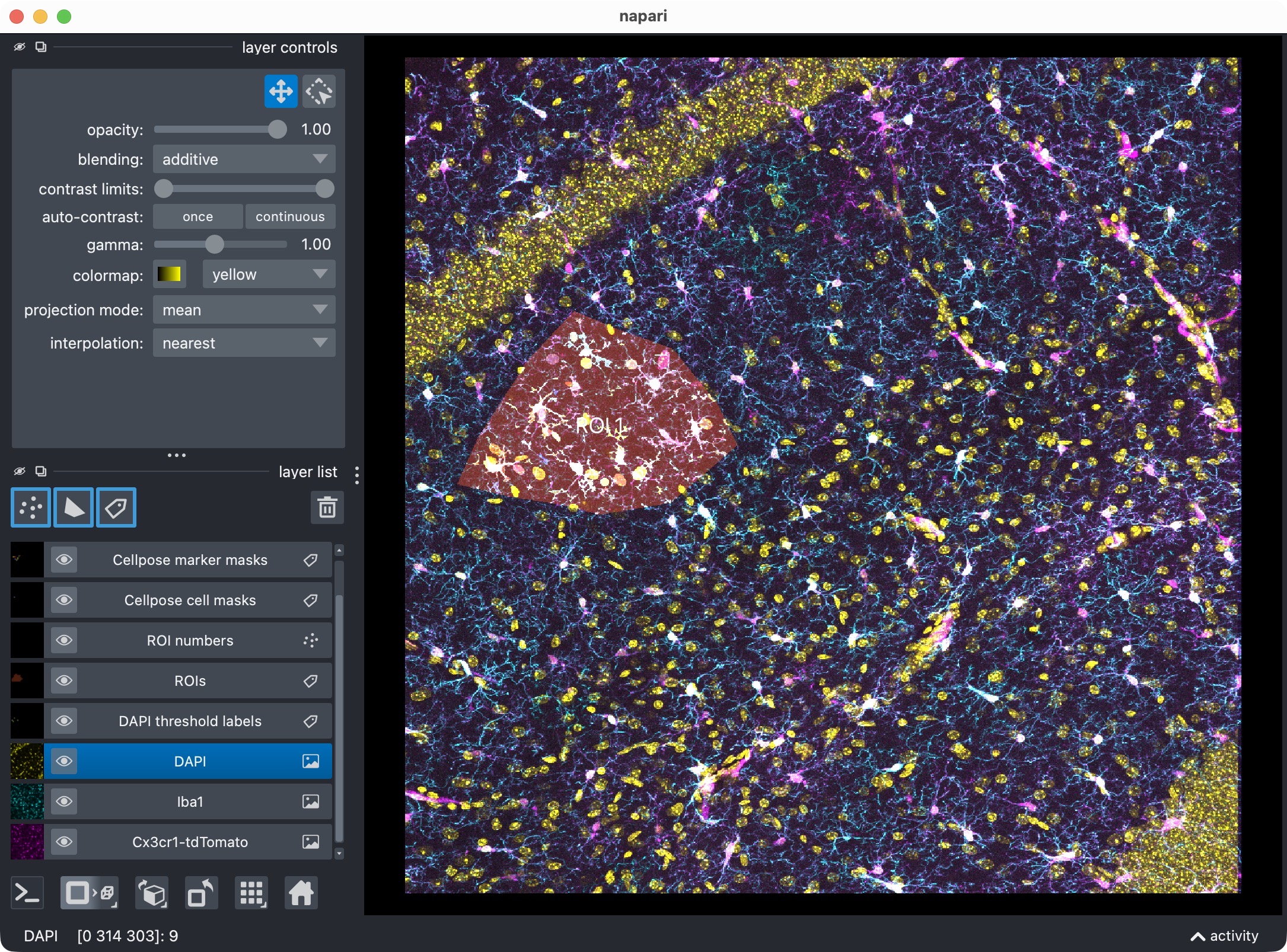
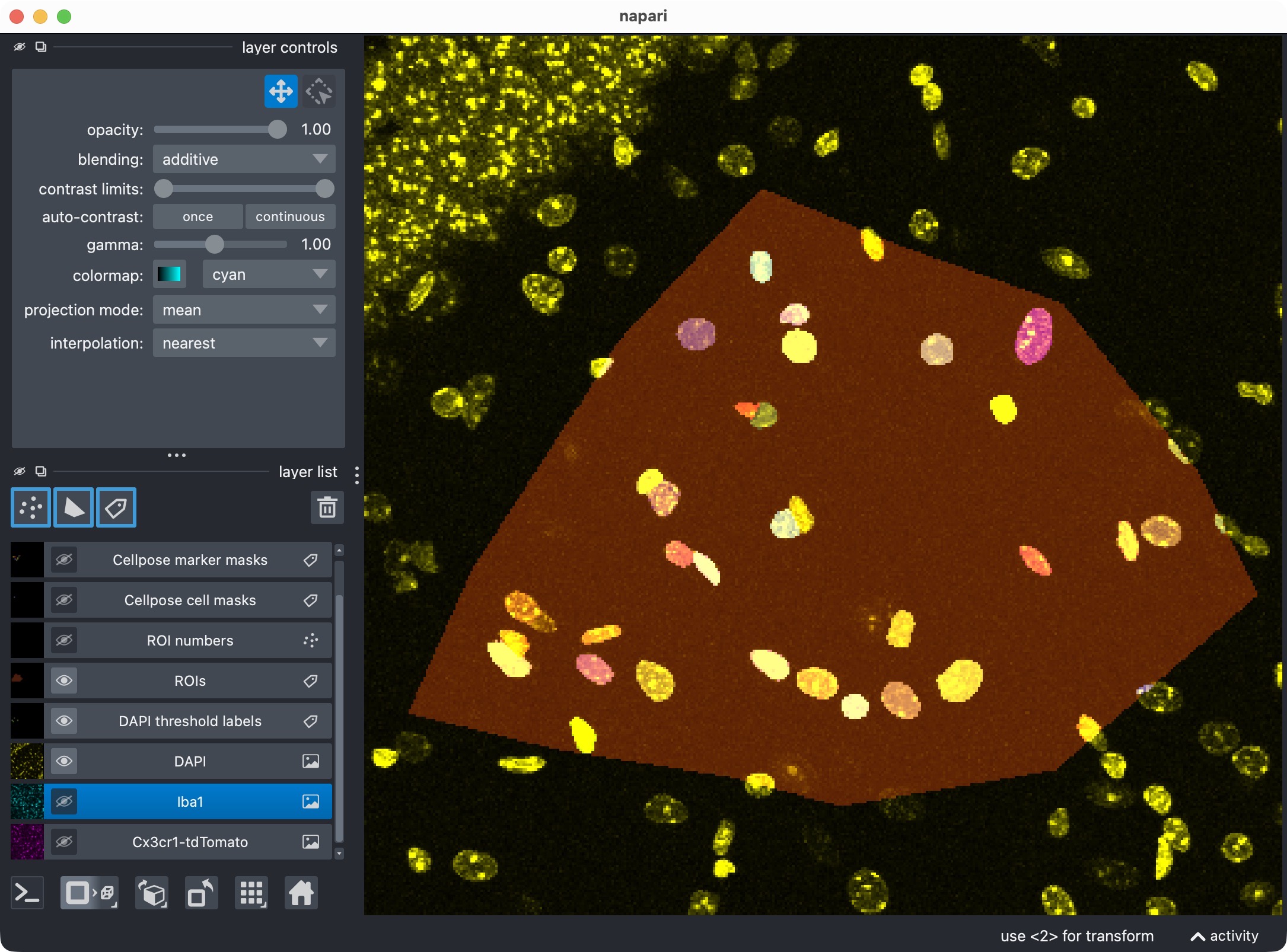
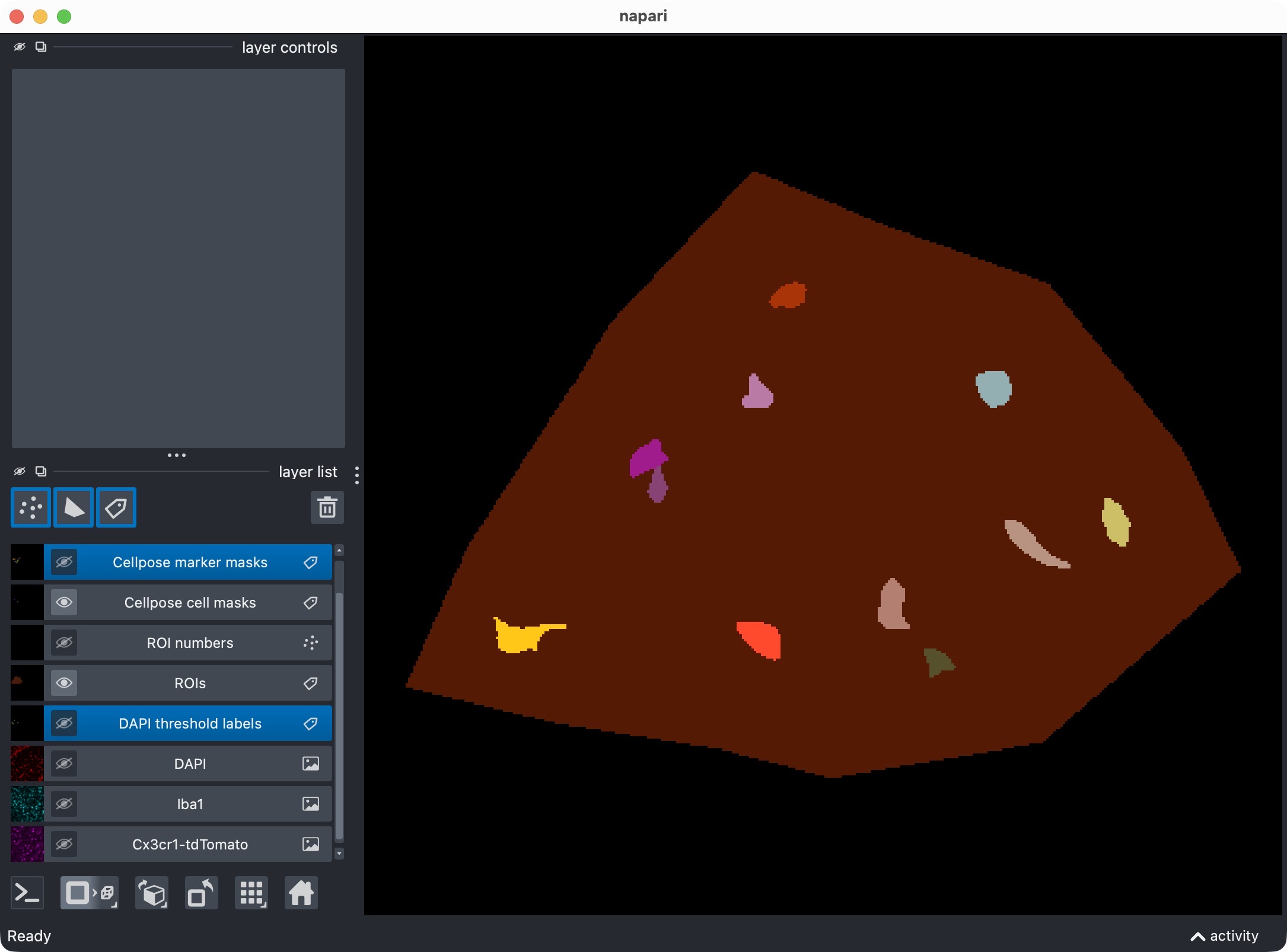
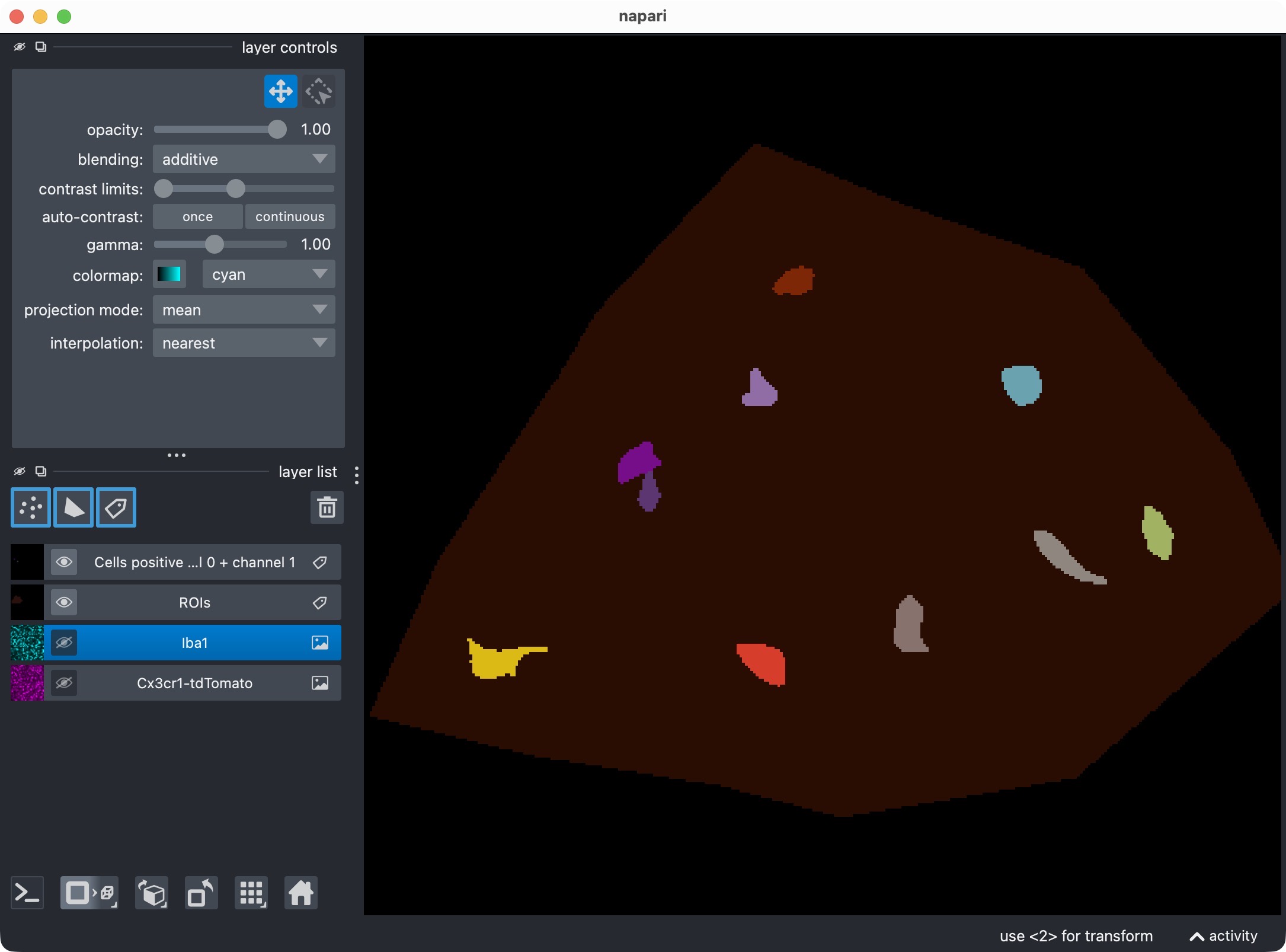
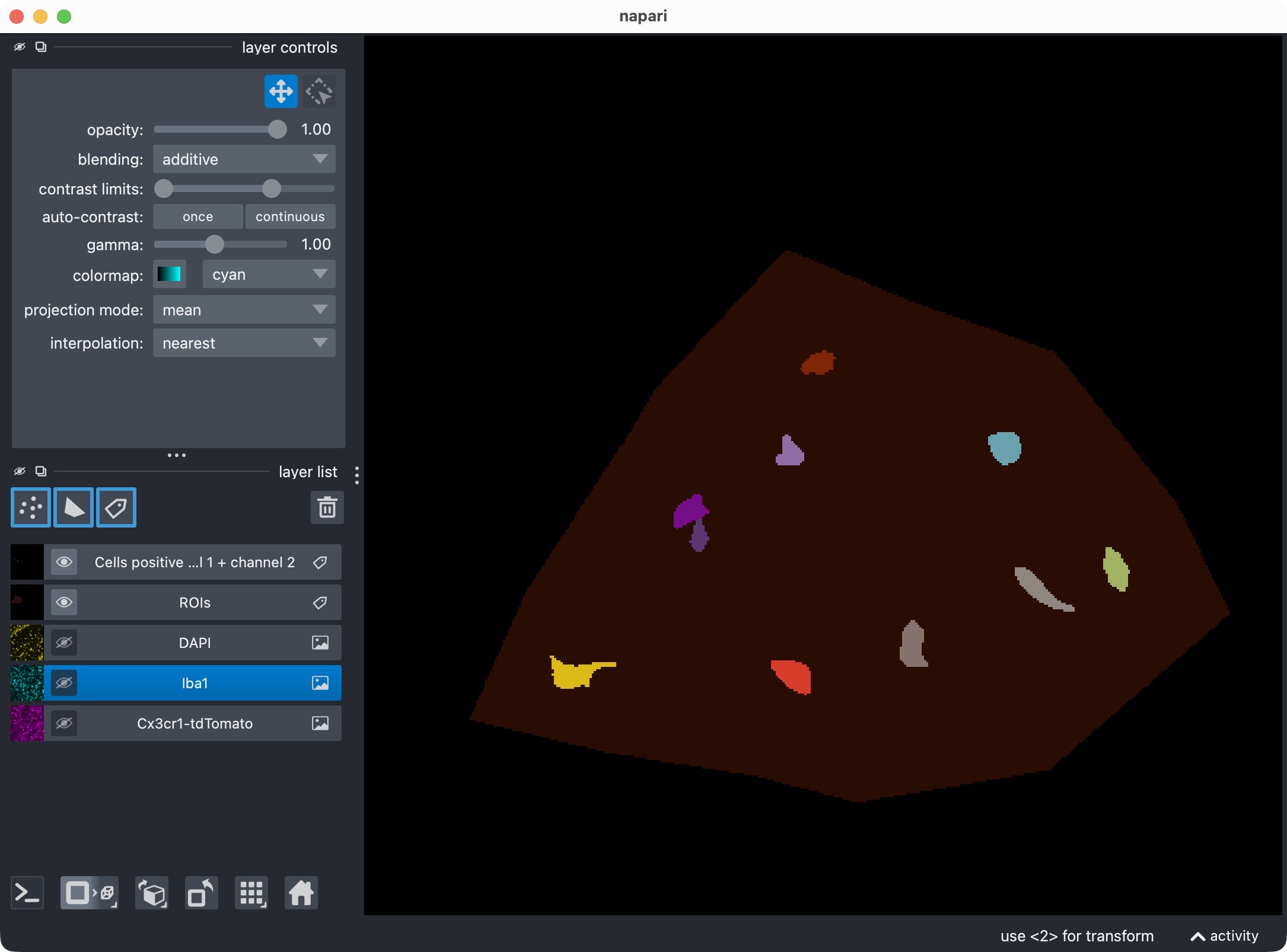
2D-projection of the original 3D stack, showing the microglia (magenta), Iba1 (cyan), and optional third channel (yellow), along with the segmentation layer of the microglia cells that are positive for both marker channels.
What you see here is no longer the original full 3D stack. Instead, CellColoc shows the projected analysis view and the corresponding segmentation layers.
This is intentional. Once you choose a z-projection, all downstream segmentation and result inspection should refer to the same projected data.
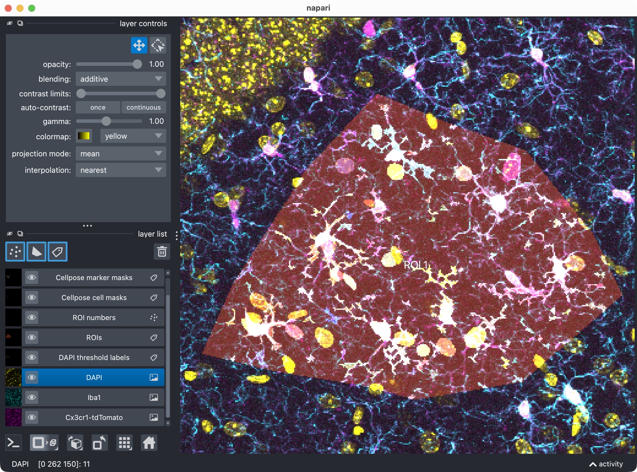
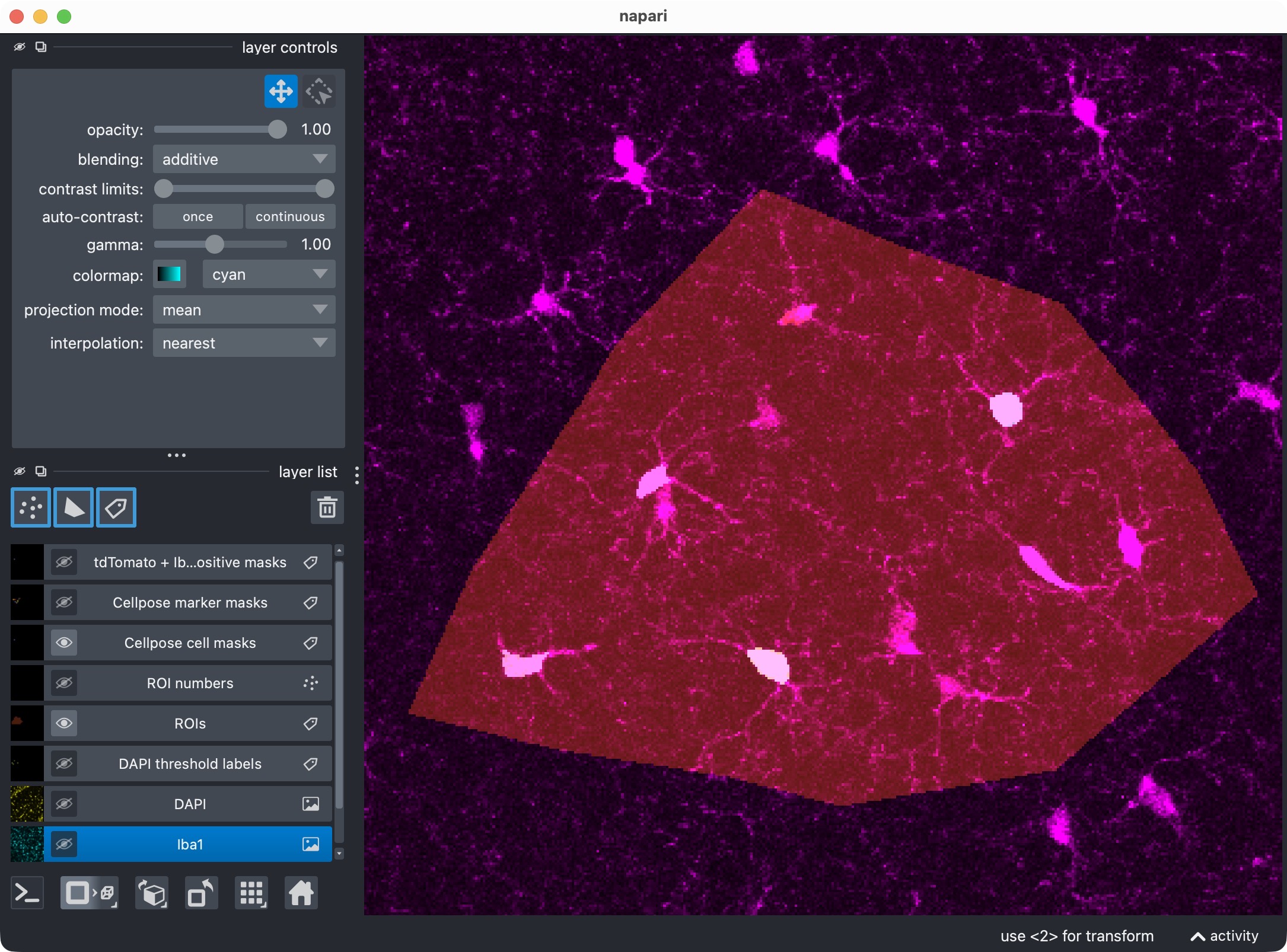
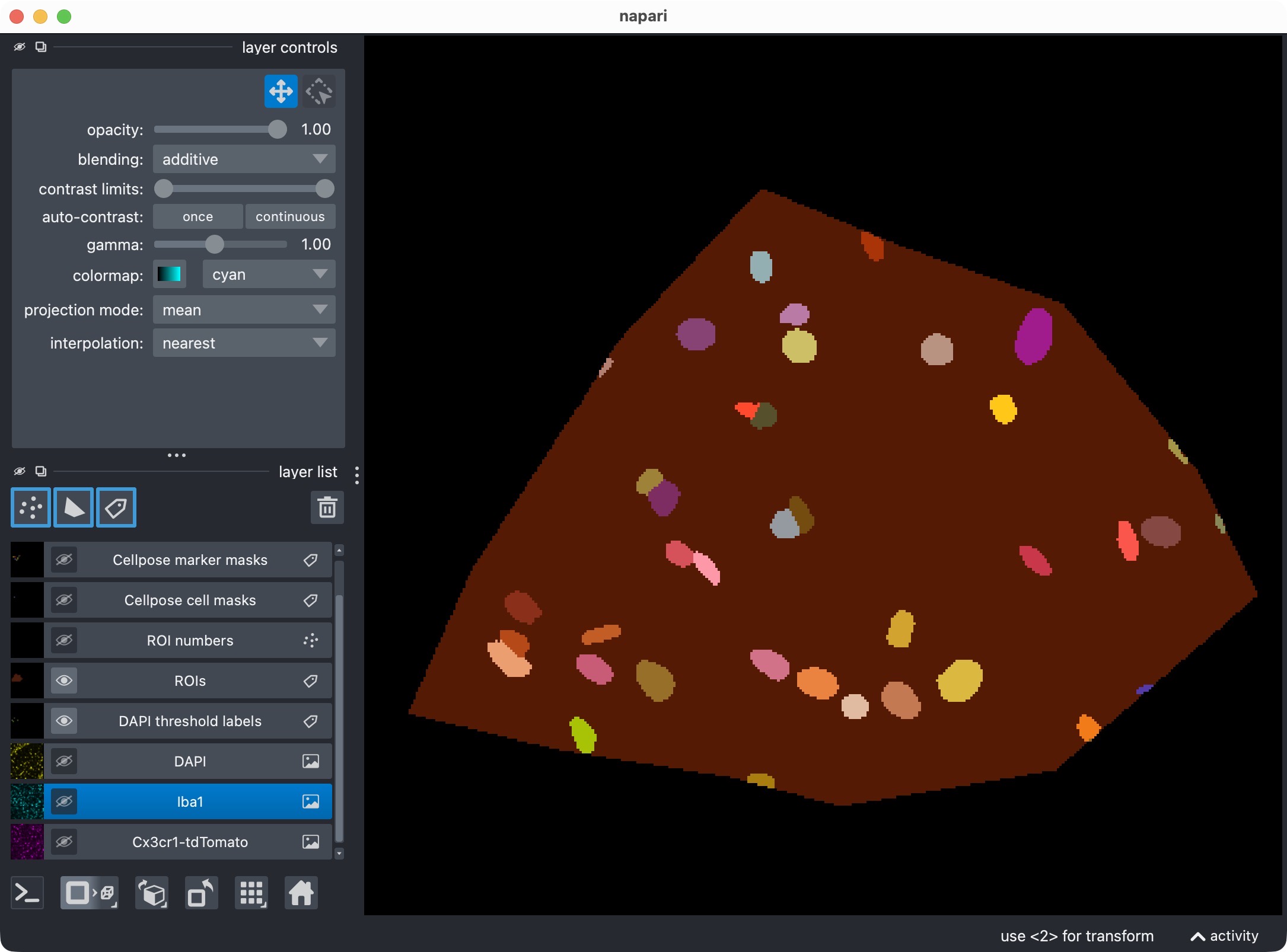
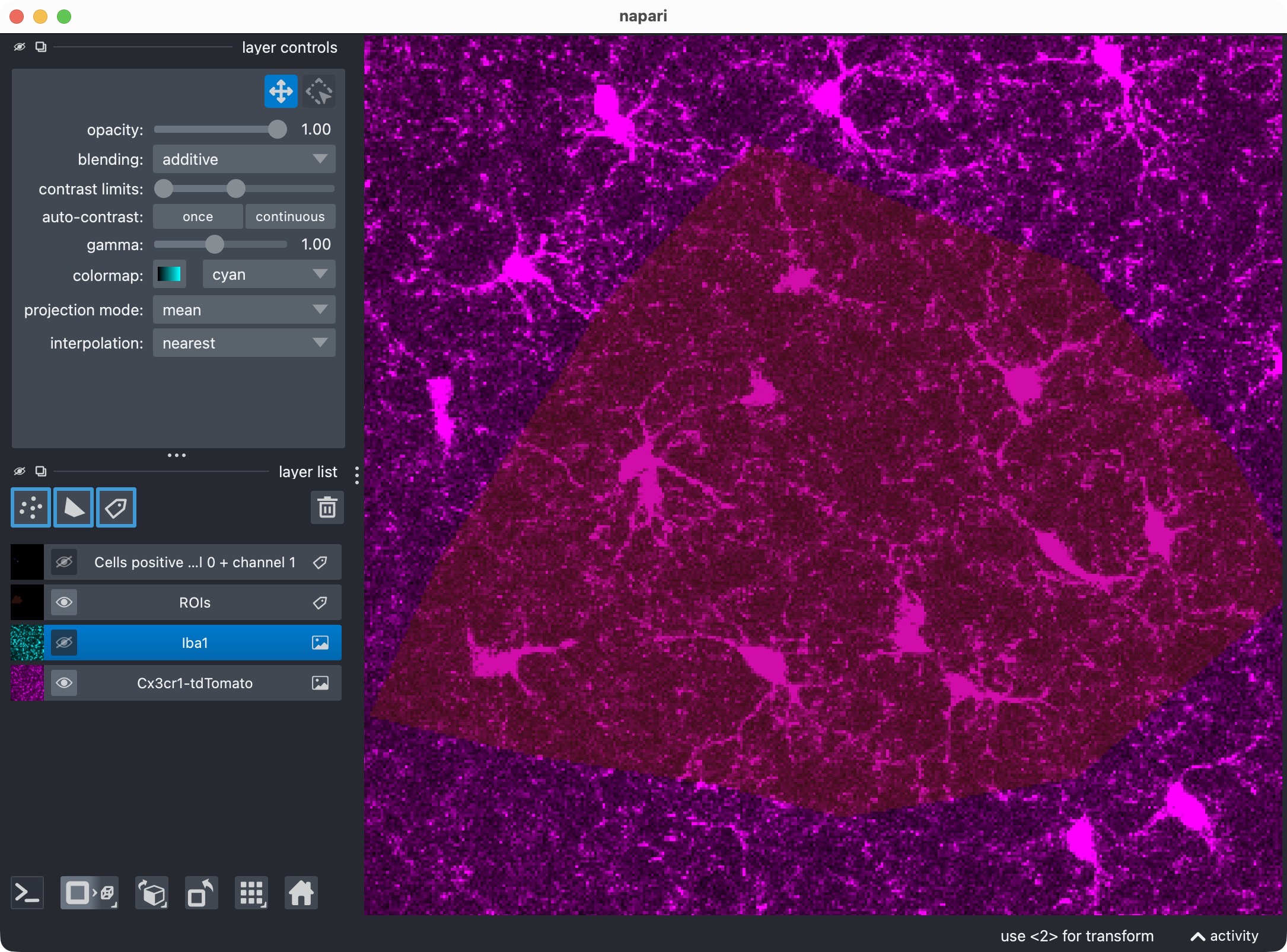
Top: Zoom onto the analyzed ROI, showing all channels and their segmented label layers. Center: Microglia channel only. Bottom: Segmentation layer of the microglia channel, showing the Cellpose-segmented cell objects. Note that we miss some microglia cells in the center of the ROI. We will try to recover them in the optional refinement step below.
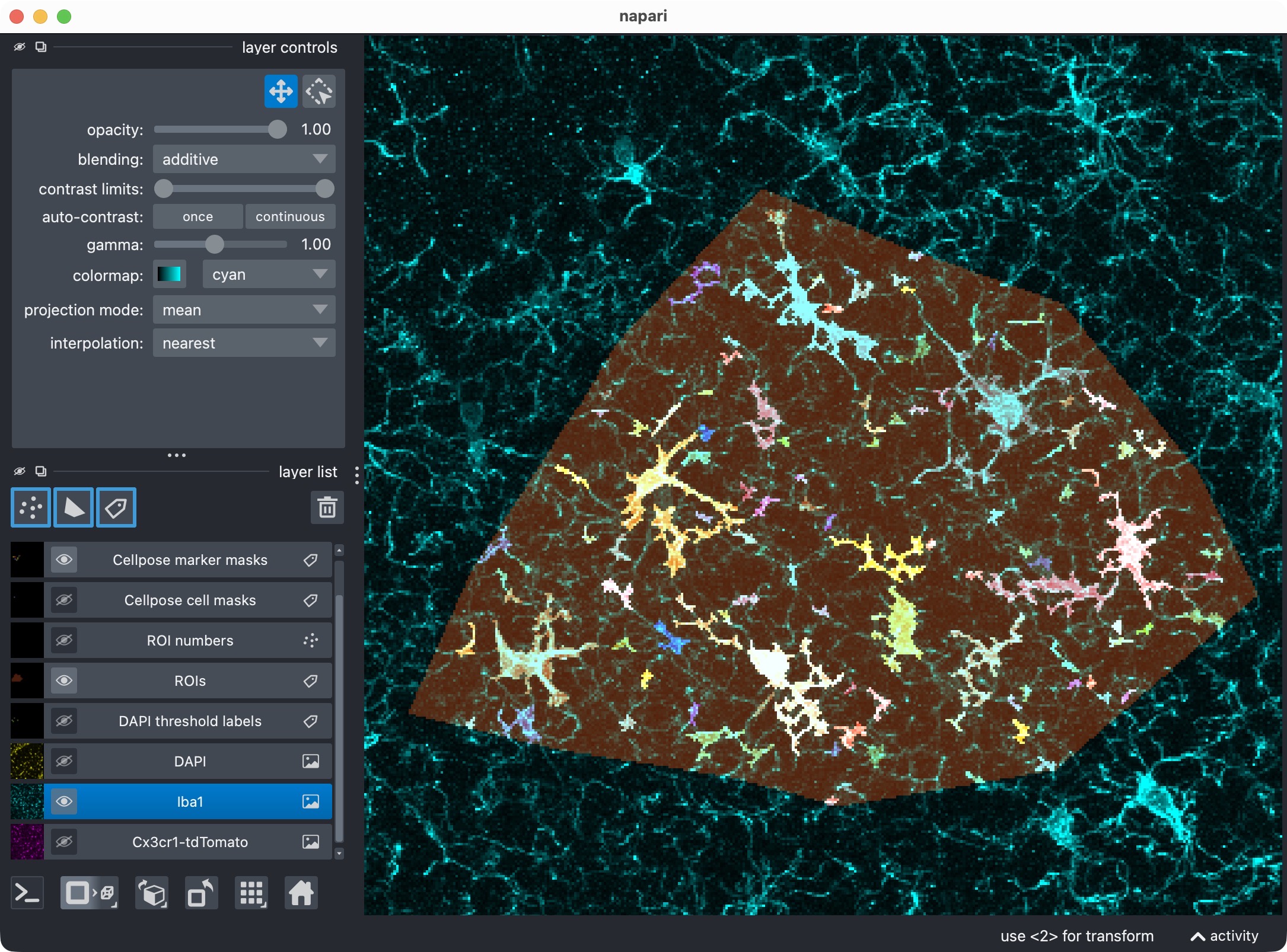
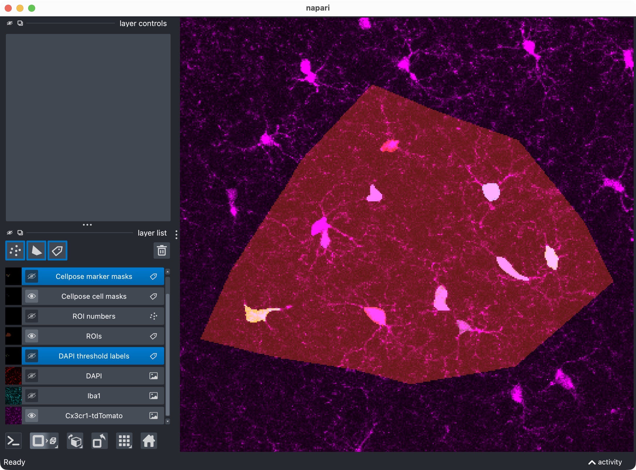
Top: Zoom onto the analyzed ROI, showing the marker channel and its segmented label layer. Bottom: Marker channel only. The marker channel is segmented with Otsu thresholding, which results in a rather rough mask. However, since we are only interested in per-cell positivity (which microglia is Iba1-positive?), this is sufficient for the current demonstration.
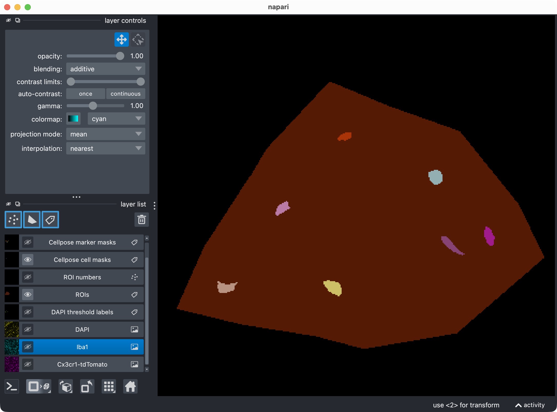
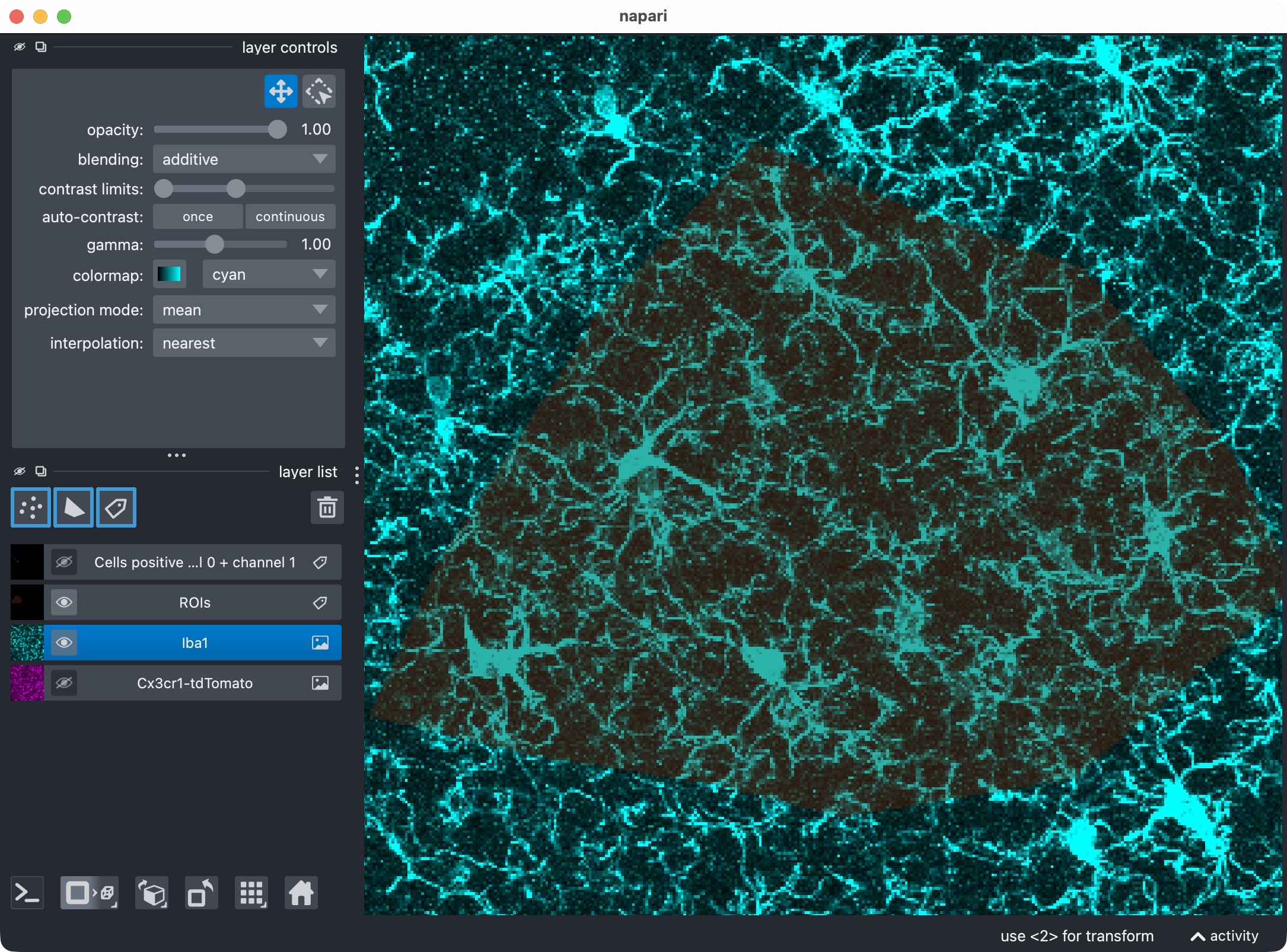
Top: Zoom onto the analyzed ROI, showing the optional third channel and its segmented label layer. Bottom: Segmented third channel only. The optional third channel is segmented with Cellpose, which results in an almost perfect mask this time. Cellpose’s segmentation quality can vary across channels and tends to work best for more “roundish” objects (the microglia’s processes complicate the Cellpose segmentation).
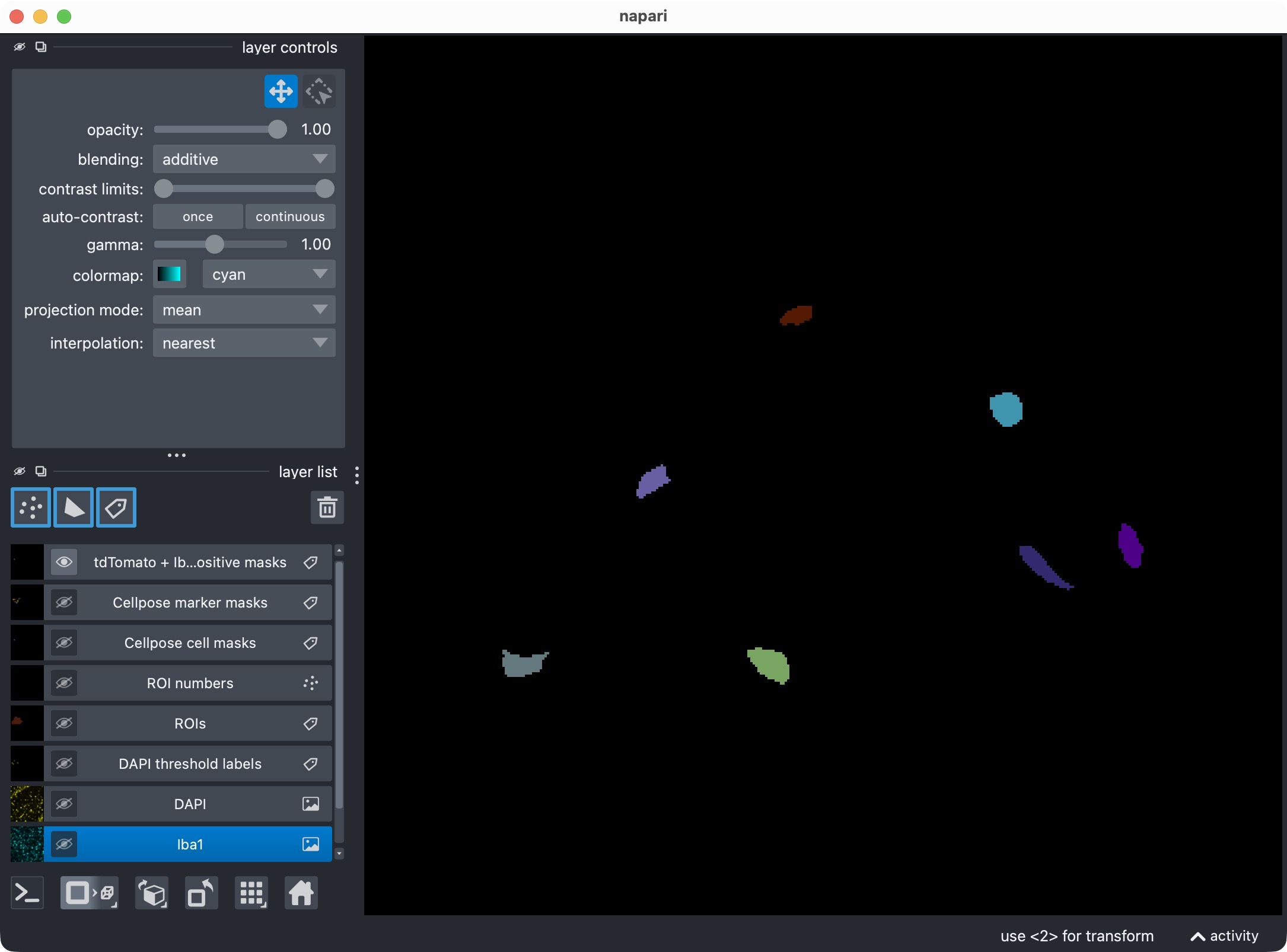
Microglia segmentation layer, including only cells that are both Iba1-positive and DAPI-positive. This is the most specific view of the three-channel analysis, showing only microglia that are positive for both marker channels. It demonstrates that the optional third channel can be used to refine the per-cell positivity analysis and create more specific subsets of cells.
Optionally refine the projected result and visualize the updated result
The next cell optionally refines the result after the first inspection:
REFINE_WITH_CACHED_CELLPOSE_OUTPUTS = True
REFINEMENT_ANALYSIS_Z_CROP = None

REFINED_CELL_CELLPROB_THRESHOLD = CELL_MODEL_CONFIG.cellprob_threshold - 1.5
REFINED_CELL_FLOW_THRESHOLD     = CELL_MODEL_CONFIG.flow_threshold -0.1

REFINED_MARKER_CELLPROB_THRESHOLD = MARKER_MODEL_CONFIG.cellprob_threshold
REFINED_MARKER_FLOW_THRESHOLD = MARKER_MODEL_CONFIG.flow_threshold

REFINED_OPTIONAL_REGION_CELLPROB_THRESHOLD = OPTIONAL_REGION_MODEL_CONFIG.cellprob_threshold
REFINED_OPTIONAL_REGION_FLOW_THRESHOLD = OPTIONAL_REGION_MODEL_CONFIG.flow_threshold

REFINED_CELL_POSTFILTERS = None
REFINED_CELL_MIN_INTENSITY_MEASURE = "mean"
REFINED_CELL_MIN_INTENSITY_THRESHOLD = None
REFINED_CELL_LOCAL_CONTRAST_K = 1.0
REFINED_CELL_LOCAL_CONTRAST_SHELL_INNER_RADIUS = 1.0
REFINED_CELL_LOCAL_CONTRAST_SHELL_OUTER_RADIUS = 4
REFINED_CELL_BRIGHT_PIXEL_MEASURE = "count"
REFINED_CELL_BRIGHT_PIXEL_THRESHOLD = None
REFINED_CELL_BRIGHT_PIXEL_MIN_COUNT = None
REFINED_CELL_BRIGHT_PIXEL_MIN_FRACTION = None

REFINED_MARKER_POSTFILTERS = None
REFINED_MARKER_MIN_INTENSITY_MEASURE = "mean"
REFINED_MARKER_MIN_INTENSITY_THRESHOLD = None
REFINED_MARKER_LOCAL_CONTRAST_K = 1.0
REFINED_MARKER_LOCAL_CONTRAST_SHELL_INNER_RADIUS = 1.0
REFINED_MARKER_LOCAL_CONTRAST_SHELL_OUTER_RADIUS = 4
REFINED_MARKER_BRIGHT_PIXEL_MEASURE = "count"
REFINED_MARKER_BRIGHT_PIXEL_THRESHOLD = None
REFINED_MARKER_BRIGHT_PIXEL_MIN_COUNT = None
REFINED_MARKER_BRIGHT_PIXEL_MIN_FRACTION = None

REFINED_OPTIONAL_REGION_POSTFILTERS = None
REFINED_OPTIONAL_REGION_MIN_INTENSITY_MEASURE = "mean"
REFINED_OPTIONAL_REGION_MIN_INTENSITY_THRESHOLD = None
REFINED_OPTIONAL_REGION_LOCAL_CONTRAST_K = 1.0
REFINED_OPTIONAL_REGION_LOCAL_CONTRAST_SHELL_INNER_RADIUS = 1.0
REFINED_OPTIONAL_REGION_LOCAL_CONTRAST_SHELL_OUTER_RADIUS = 4
REFINED_OPTIONAL_REGION_BRIGHT_PIXEL_MEASURE = "count"
REFINED_OPTIONAL_REGION_BRIGHT_PIXEL_THRESHOLD = None
REFINED_OPTIONAL_REGION_BRIGHT_PIXEL_MIN_COUNT = None
REFINED_OPTIONAL_REGION_BRIGHT_PIXEL_MIN_FRACTION = None

effective_refinement_z_crop = (
    CELL_MODEL_CONFIG.z_crop if REFINEMENT_ANALYSIS_Z_CROP is None else REFINEMENT_ANALYSIS_Z_CROP)

if REFINE_WITH_CACHED_CELLPOSE_OUTPUTS:
    refined_cell_model_config = replace(
        CELL_MODEL_CONFIG,
        z_crop=effective_refinement_z_crop,
        postfilters=REFINED_CELL_POSTFILTERS,
        min_intensity_measure=REFINED_CELL_MIN_INTENSITY_MEASURE,
        min_intensity_threshold=REFINED_CELL_MIN_INTENSITY_THRESHOLD,
        local_contrast_k=REFINED_CELL_LOCAL_CONTRAST_K,
        local_contrast_shell_inner_radius=REFINED_CELL_LOCAL_CONTRAST_SHELL_INNER_RADIUS,
        local_contrast_shell_outer_radius=REFINED_CELL_LOCAL_CONTRAST_SHELL_OUTER_RADIUS,
        bright_pixel_measure=REFINED_CELL_BRIGHT_PIXEL_MEASURE,
        bright_pixel_threshold=REFINED_CELL_BRIGHT_PIXEL_THRESHOLD,
        bright_pixel_min_count=REFINED_CELL_BRIGHT_PIXEL_MIN_COUNT,
        bright_pixel_min_fraction=REFINED_CELL_BRIGHT_PIXEL_MIN_FRACTION)
    refined_marker_model_config = replace(
        MARKER_MODEL_CONFIG,
        z_crop=effective_refinement_z_crop,
        postfilters=REFINED_MARKER_POSTFILTERS,
        min_intensity_measure=REFINED_MARKER_MIN_INTENSITY_MEASURE,
        min_intensity_threshold=REFINED_MARKER_MIN_INTENSITY_THRESHOLD,
        local_contrast_k=REFINED_MARKER_LOCAL_CONTRAST_K,
        local_contrast_shell_inner_radius=REFINED_MARKER_LOCAL_CONTRAST_SHELL_INNER_RADIUS,
        local_contrast_shell_outer_radius=REFINED_MARKER_LOCAL_CONTRAST_SHELL_OUTER_RADIUS,
        bright_pixel_measure=REFINED_MARKER_BRIGHT_PIXEL_MEASURE,
        bright_pixel_threshold=REFINED_MARKER_BRIGHT_PIXEL_THRESHOLD,
        bright_pixel_min_count=REFINED_MARKER_BRIGHT_PIXEL_MIN_COUNT,
        bright_pixel_min_fraction=REFINED_MARKER_BRIGHT_PIXEL_MIN_FRACTION)
    refined_optional_region_model_config = replace(
        OPTIONAL_REGION_MODEL_CONFIG,
        z_crop=effective_refinement_z_crop,
        postfilters=REFINED_OPTIONAL_REGION_POSTFILTERS,
        min_intensity_measure=REFINED_OPTIONAL_REGION_MIN_INTENSITY_MEASURE,
        min_intensity_threshold=REFINED_OPTIONAL_REGION_MIN_INTENSITY_THRESHOLD,
        local_contrast_k=REFINED_OPTIONAL_REGION_LOCAL_CONTRAST_K,
        local_contrast_shell_inner_radius=REFINED_OPTIONAL_REGION_LOCAL_CONTRAST_SHELL_INNER_RADIUS,
        local_contrast_shell_outer_radius=REFINED_OPTIONAL_REGION_LOCAL_CONTRAST_SHELL_OUTER_RADIUS,
        bright_pixel_measure=REFINED_OPTIONAL_REGION_BRIGHT_PIXEL_MEASURE,
        bright_pixel_threshold=REFINED_OPTIONAL_REGION_BRIGHT_PIXEL_THRESHOLD,
        bright_pixel_min_count=REFINED_OPTIONAL_REGION_BRIGHT_PIXEL_MIN_COUNT,
        bright_pixel_min_fraction=REFINED_OPTIONAL_REGION_BRIGHT_PIXEL_MIN_FRACTION)

    run_result = refine_run_result_from_cellpose_cache(
        loaded_images=loaded_images,
        roi_labels_2d=roi_labels_2d,
        run_result=run_result,
        colocalization_config=COLOCALIZATION_CONFIG,
        cell_model_config=refined_cell_model_config,
        marker_model_config=None,
        optional_region_model_config=refined_optional_region_model_config,
        cell_cellprob_threshold=REFINED_CELL_CELLPROB_THRESHOLD,
        cell_flow_threshold=REFINED_CELL_FLOW_THRESHOLD,
        marker_cellprob_threshold=REFINED_MARKER_CELLPROB_THRESHOLD,
        marker_flow_threshold=REFINED_MARKER_FLOW_THRESHOLD,
        optional_region_cellprob_threshold=REFINED_OPTIONAL_REGION_CELLPROB_THRESHOLD,
        optional_region_flow_threshold=REFINED_OPTIONAL_REGION_FLOW_THRESHOLD,
        optional_region_result=None)

    print("Projected refinement finished. "
          f"Overview rows: {len(run_result.tables.overview)}, "
          f"summary rows: {len(run_result.tables.summary)}.")

    if RUNTIME_CONFIG.open_results:
        result_viewer = show_analysis_results(
            loaded_images=loaded_images,
            roi_labels_2d=roi_labels_2d,
            run_result=run_result,
            display_names=DISPLAY_NAMES,
            optional_region_result=None,
            viewer=result_viewer,
            layers_to_show=REFINEMENT_RESULT_LAYER_KEYS,
            replace_existing_layers=True,
            show_optional_region_image=True)

        print(f"Inspecting refined visualization for:\n{SELECTED_FILE_NAME}")
        napari.run()
else:
    print("Cached Cellpose refinement is disabled for this run.")
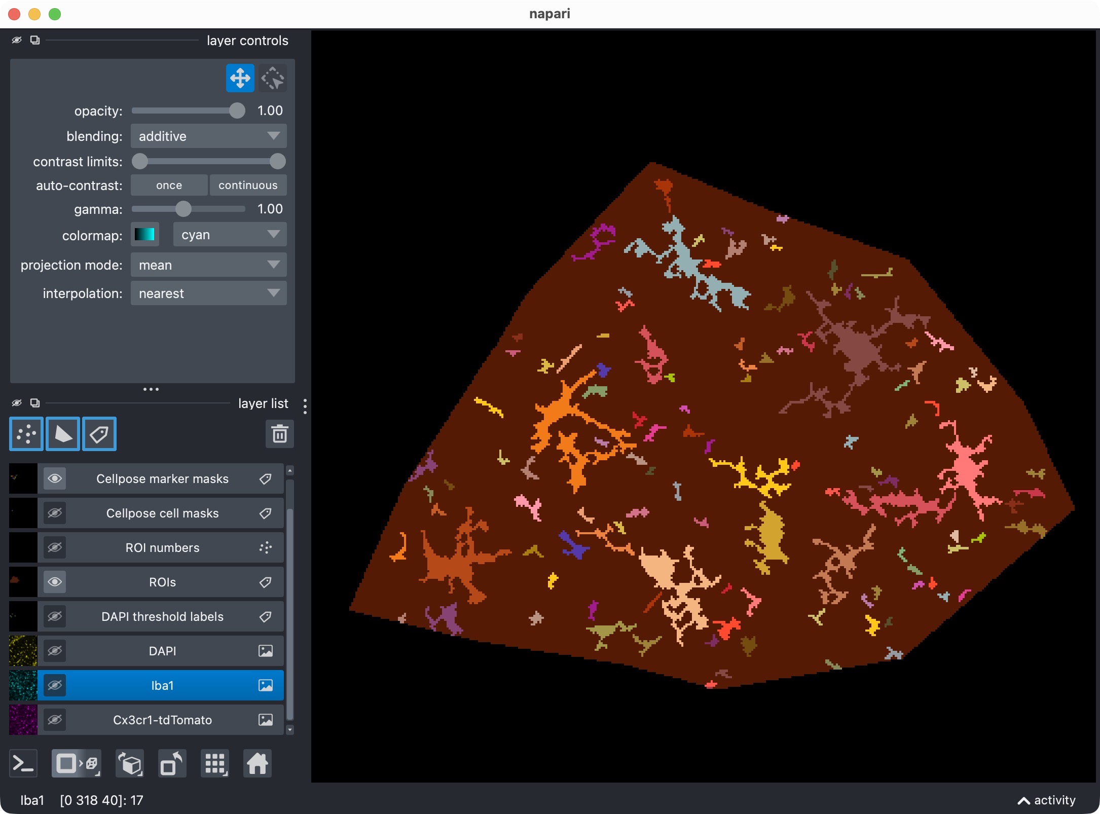
Refinement results for the microglia channel. Initially, the Cellpose segmentation of the microglia channel missed some cells in the center of the ROI. By activating the refinement block, we can recover some of these missed cells without having to rerun the full initial segmentation. The refinement uses cached Cellpose outputs to adjust the segmentation masks post hoc.
This refinement block serves two purposes:
it lets you tighten or relax Cellpose-derived masks without rerunning the full initial segmentation,
and it shows that the projected workflow can still be refined interactively.
In the current script:
the cell channel can be refined through cached Cellpose outputs,
the third channel can also be refined because it was initially segmented with Cellpose,
the marker channel keeps its original Otsu-based segmentation in the current demo, because threshold-based channels do not provide Cellpose refinement caches.
Important settings
REFINE_WITH_CACHED_CELLPOSE_OUTPUTSmaster switch for the refinement step.
REFINEMENT_ANALYSIS_Z_CROPoptional z interval that is applied before projection for the refinement run. If left as
None, the original projection span is reused.REFINED_*_CELLPROB_THRESHOLDandREFINED_*_FLOW_THRESHOLDCellpose threshold parameters for the channels that were initially segmented with Cellpose.
REFINED_*_POSTFILTERSoptional post hoc filters such as
"min_intensity","local_contrast", or"bright_pixel_support". In this projected demonstration script they are left atNoneby default.
The block already contains the full parameter structure, so you can activate these filters later without having to rewrite the workflow.
Optionally reanalyze manually edited label layers from napari
If you edit the label layers manually in napari, the next cell can rebuild the tables from your edited masks:
REANALYZE_EDITED_LABELS_FROM_VIEWER = False

if REANALYZE_EDITED_LABELS_FROM_VIEWER:
    cell_masks_from_viewer, marker_masks_from_viewer = extract_label_masks_from_viewer(result_viewer)
    run_result = analyze_existing_masks(
        loaded_images=loaded_images,
        roi_labels_2d=roi_labels_2d,
        cell_masks=cell_masks_from_viewer,
        marker_masks=marker_masks_from_viewer,
        colocalization_config=COLOCALIZATION_CONFIG,
        optional_region_result=None,
        optional_region_masks=run_result.optional_region_masks,
        analysis_z_bounds=run_result.analysis_z_bounds,
        cell_refinement_context=run_result.cell_refinement_context,
        marker_refinement_context=run_result.marker_refinement_context,
        optional_region_refinement_context=run_result.optional_region_refinement_context)

    result_viewer = show_analysis_results(
        loaded_images=loaded_images,
        roi_labels_2d=roi_labels_2d,
        run_result=run_result,
        display_names=DISPLAY_NAMES,
        optional_region_result=None,
        viewer=result_viewer,
        layers_to_show=REFINEMENT_RESULT_LAYER_KEYS,
        replace_existing_layers=True,
        show_optional_region_image=True)
    print("Inspect the relabeled result in napari and close the window when finished.")
    napari.run()
else:
    print("Manual label reanalysis from the napari viewer is disabled for this run.")

roi_display_labels = np.broadcast_to(roi_labels_2d, loaded_images.cell_image.shape).copy()
This is useful when:
you want to merge or split labels manually using napari’s label editing tools,
you want to remove obvious segmentation artifacts by hand,
or you want to produce a final polished result table from curated masks.
The reanalysis uses the currently displayed label layers from the open napari viewer rather than loading masks from disk.
Visualize cells positive for channel 0 + channel 1
The next cell creates a dedicated positivity view for channel 0 against channel 1:
summary_channel01 = run_result.tables.summary.copy()
summary_channel01["marker_positive"] = summary_channel01["marker_positive"].astype(bool)
channel01_positive_masks = build_positive_cell_mask(run_result.cell_masks, summary_channel01)

viewer_01 = napari.Viewer()
viewer_01.add_image(
    loaded_images.cell_image,
    name=DISPLAY_NAMES.cell,
    scale=loaded_images.voxel_scale_zyx,
    blending="additive",
    colormap="magenta")
viewer_01.add_image(
    loaded_images.marker_image,
    name=DISPLAY_NAMES.marker,
    scale=loaded_images.voxel_scale_zyx,
    blending="additive",
    colormap="cyan")
viewer_01.add_labels(
    roi_display_labels,
    name="ROIs",
    scale=loaded_images.voxel_scale_zyx,
    opacity=0.35)
viewer_01.add_labels(
    channel01_positive_masks,
    name="Cells positive for channel 0 + channel 1",
    scale=loaded_images.voxel_scale_zyx,
    blending="additive")
print("Inspect channel-0 plus channel-1 positive cells.")
napari.run()
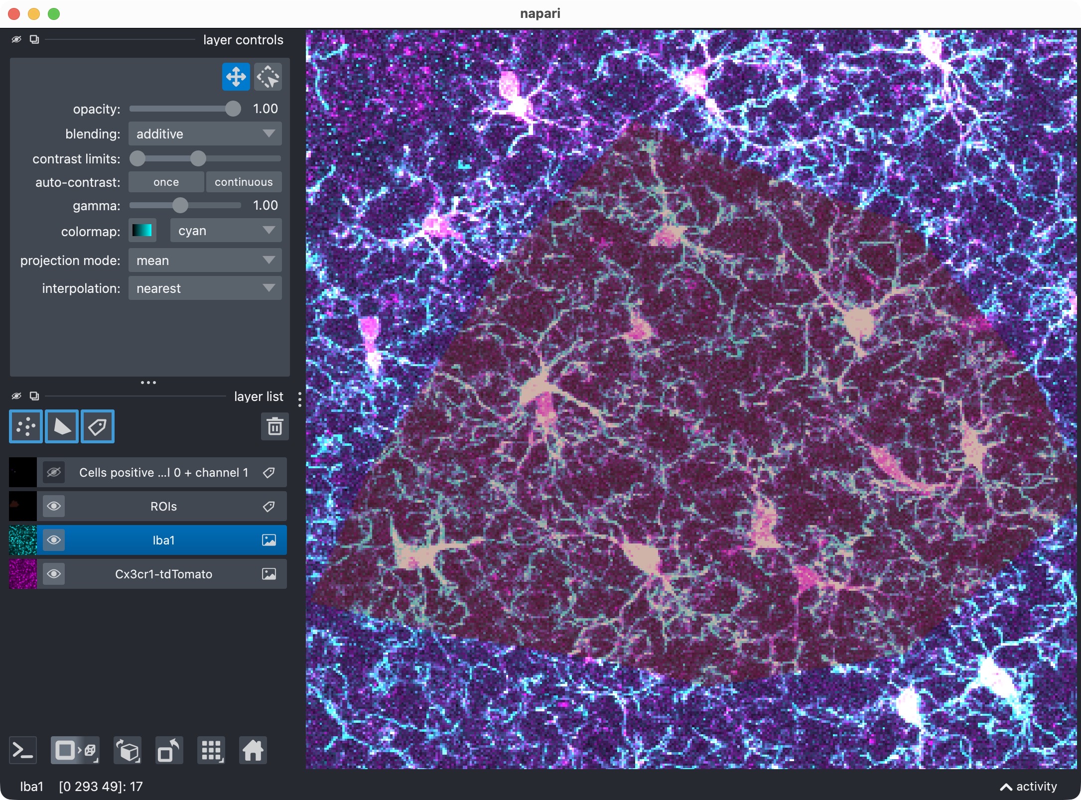
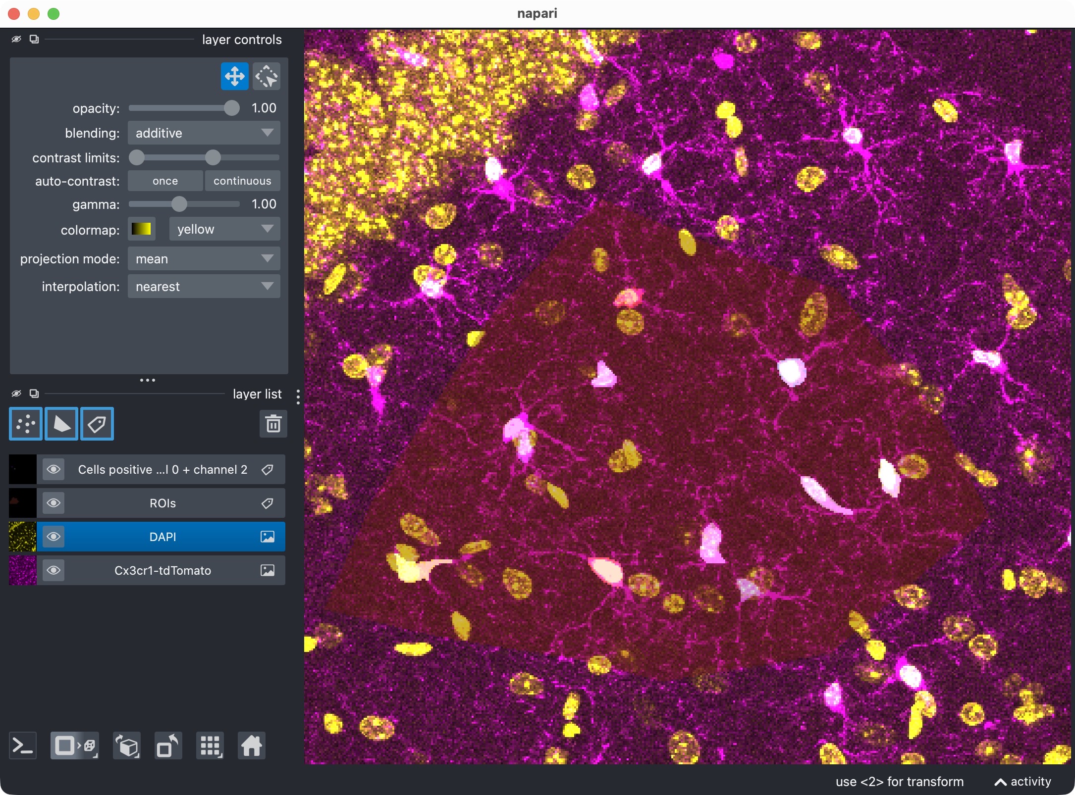
Top: Zoom onto the analyzed ROI, showing the microglia, Iba1, and the resulting segmentation layer of the microglia cells that are positive for Iba1. Center top: The microglia channel only. Center bottom: The Iba1 channel only. Bottom: Segmentation layer of the Iba1-positive cells. This view shows which microglia cells are positive for the Iba1 marker, based on the projected analysis and segmentation results.
This view shows:
the projected cell image,
the projected marker image,
the ROI layer,
and only those channel-0 cell masks that are positive against channel 1.
Visualize cells positive for channel 0 + channel 2
The following cell creates the dedicated positivity view for channel 0 against channel 2:
summary_channel02 = run_result.tables.summary.copy()
summary_channel02["marker_positive"] = summary_channel02["optional_region_positive"].astype(bool)
channel02_positive_masks = build_positive_cell_mask(run_result.cell_masks, summary_channel02)

viewer_02 = napari.Viewer()
viewer_02.add_image(
    loaded_images.cell_image,
    name=DISPLAY_NAMES.cell,
    scale=loaded_images.voxel_scale_zyx,
    blending="additive",
    colormap="magenta")
viewer_02.add_image(
    loaded_images.optional_region_image,
    name=DISPLAY_NAMES.optional_region,
    scale=loaded_images.voxel_scale_zyx,
    blending="additive",
    colormap="yellow")
viewer_02.add_labels(
    roi_display_labels,
    name="ROIs",
    scale=loaded_images.voxel_scale_zyx,
    opacity=0.35)
viewer_02.add_labels(
    channel02_positive_masks,
    name="Cells positive for channel 0 + channel 2",
    scale=loaded_images.voxel_scale_zyx,
    blending="additive")
print("Inspect channel-0 plus channel-2 positive cells.")
napari.run()
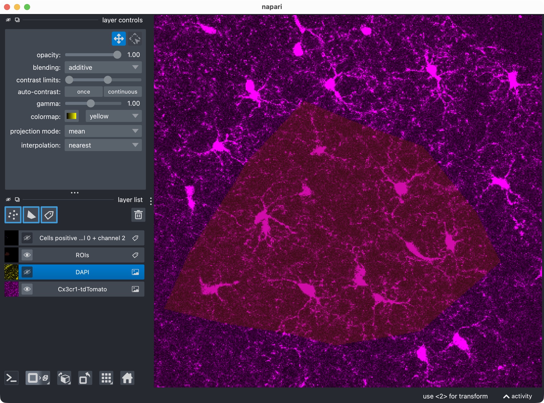
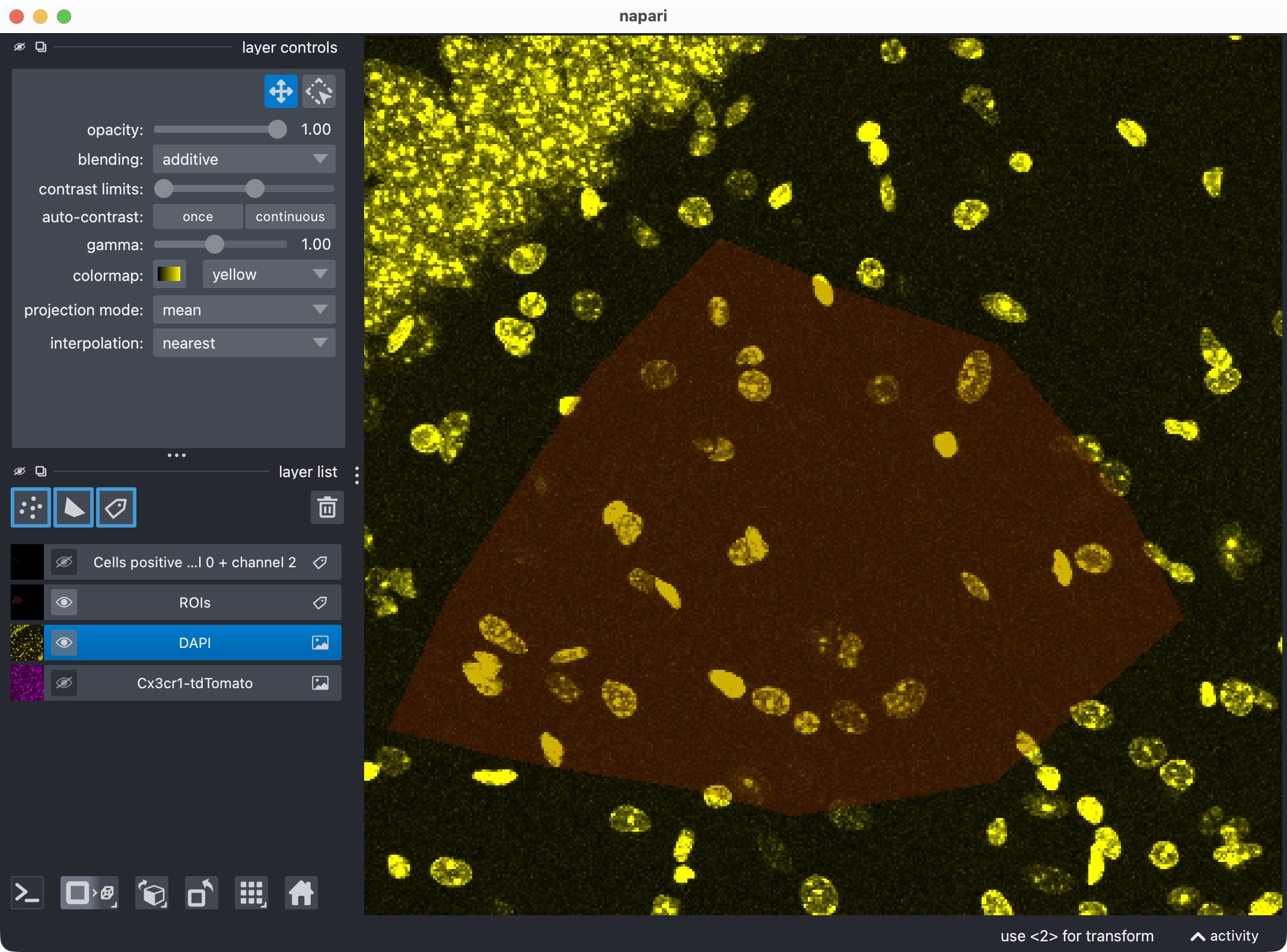
Top: Zoom onto the analyzed ROI, showing the microglia, DAPI, and the resulting segmentation layer of the microglia cells that are positive for DAPI. Center top: The microglia channel only. Center bottom: The DAPI channel only. Bottom: Segmentation layer of the DAPI-positive cells. This view shows which microglia cells are positive for the DAPI marker, based on the projected analysis and segmentation results.
This is the optional-third-channel analogue of the previous view.
Visualize cells positive for channel 0 + channel 1 + channel 2
The next cell creates the combined double-positive view:
summary_channel012 = run_result.tables.summary.copy()
summary_channel012["marker_positive"] = summary_channel012["marker_and_optional_region_positive"].astype(bool)
channel012_positive_masks = build_positive_cell_mask(run_result.cell_masks, summary_channel012)

viewer_012 = napari.Viewer()
viewer_012.add_image(
    loaded_images.cell_image,
    name=DISPLAY_NAMES.cell,
    scale=loaded_images.voxel_scale_zyx,
    blending="additive",
    colormap="magenta")
viewer_012.add_image(
    loaded_images.marker_image,
    name=DISPLAY_NAMES.marker,
    scale=loaded_images.voxel_scale_zyx,
    blending="additive",
    colormap="cyan")
viewer_012.add_image(
    loaded_images.optional_region_image,
    name=DISPLAY_NAMES.optional_region,
    scale=loaded_images.voxel_scale_zyx,
    blending="additive",
    colormap="yellow")
viewer_012.add_labels(
    roi_display_labels,
    name="ROIs",
    scale=loaded_images.voxel_scale_zyx,
    opacity=0.35)
viewer_012.add_labels(
    channel012_positive_masks,
    name="Cells positive for channel 0 + channel 1 + channel 2",
    scale=loaded_images.voxel_scale_zyx,
    blending="additive")
print("Inspect channel-0 plus channel-1 plus channel-2 positive cells.")
napari.run()
Top: Zoom onto the analyzed ROI, showing the microglia, Iba1, DAPI, and the resulting segmentation layer of the microglia cells that are positive for both Iba1 and DAPI. Bottom: Segmentation layer of the Iba1- and DAPI-positive cells.
This final positivity view is often the most biologically restrictive one. It shows only those channel-0 cells that satisfy both positivity conditions at the same time.
Export results
The last cell exports the final run result:
export_analysis_outputs(
    run_result=run_result,
    paths=loaded_images.paths,
    optional_region_result=None)
print("Final results exported.")
This writes the standard CellColoc outputs to the results/ directory
associated with the current input file, including:
exported masks,
ROI masks,
summary tables,
and the Excel workbook with the main analysis results.
At this point, the projected three-channel workflow is complete.