3D data analysis tutorial
This tutorial walks through a complete 3D CellColoc workflow based on the interactive Jupyter notebook
user_scripts/nb_microglia_3D_user_script.ipynb,
which is identical to the interactive Python script
user_scripts/microglia_3D_user_script.py.
The goal is to show how to analyze a multichannel 3D microscopy stack from scratch, how to configure CellColoc for interactive ROI-based 3D analysis, and how to use 3D-specific features such as pre-filtering strategies, anisotropy handling, disk-backed loading, global z-cropping, cache-based refinement including post-filtering, and manual relabel-based reanalyis.
Dataset used in this tutorial
The tutorial uses the microglia example data set distributed with CellColoc in
example_data/microglia_3D/
Please download the example data from the CellColoc Zenodo example-data record first, as described in the Example data set section. Store the downloaded files locally in a convenient place. For the remainder of this tutorial, we assume that the downloaded files are available relative to the current working directory or current example script in:
example_data/microglia_3D/
The script is written to handle one selected file from that folder at a time.
This is a real 3D multichannel fluorescence dataset. In this tutorial, we treat:
channel 0 as the primary
cellchannel (Cx3cr1-tdTomatomicroglia reporter signal),channel 1 as the primary
markerchannel (Iba1staining),channel 2 as an additional image channel for orientation and optional visualization (
DAPI).
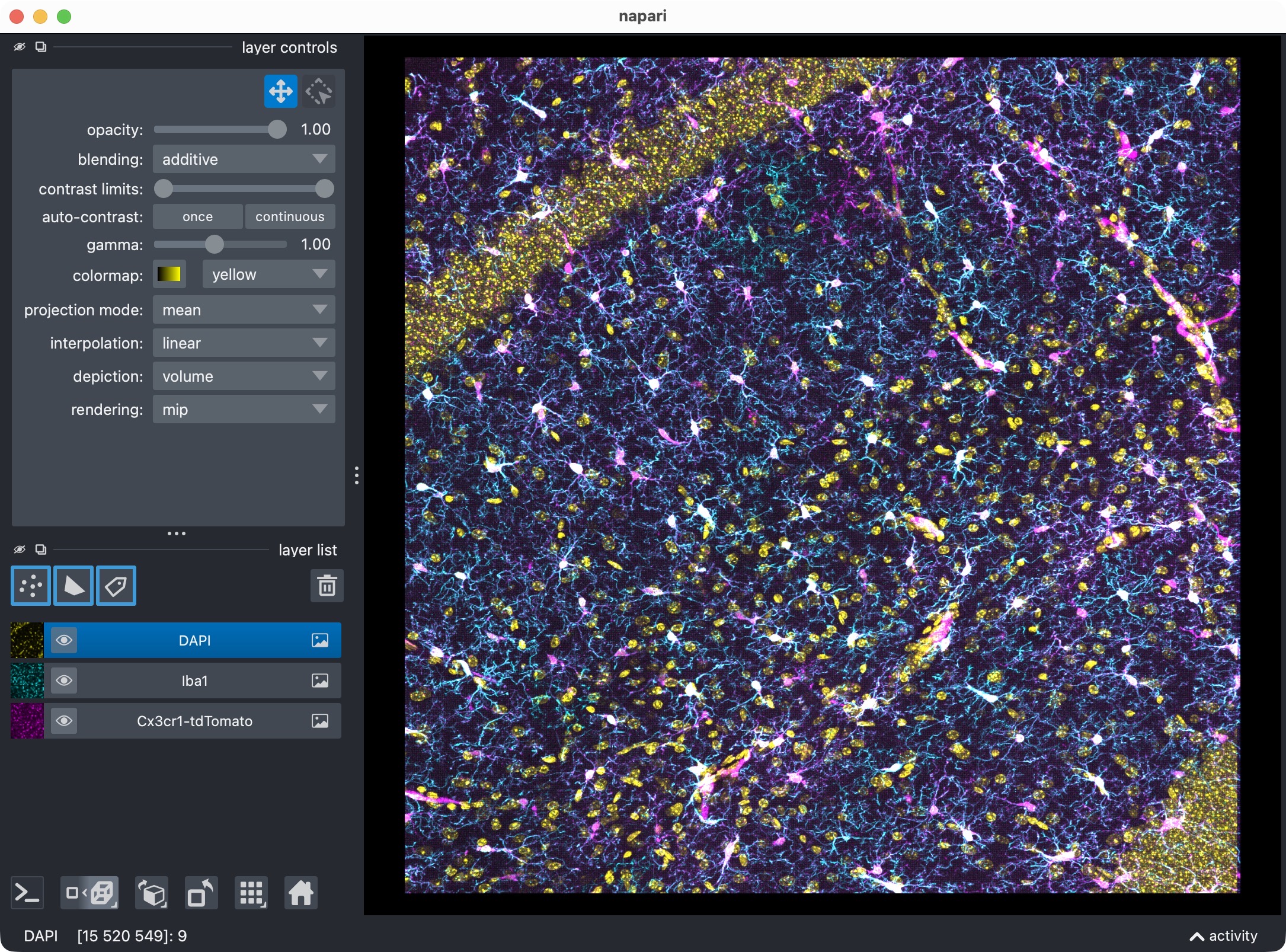
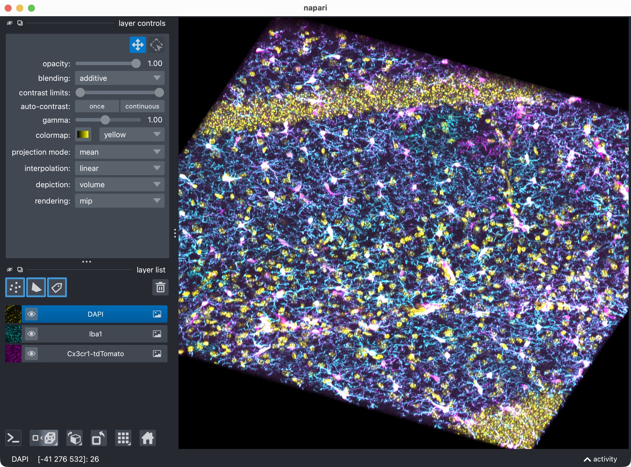
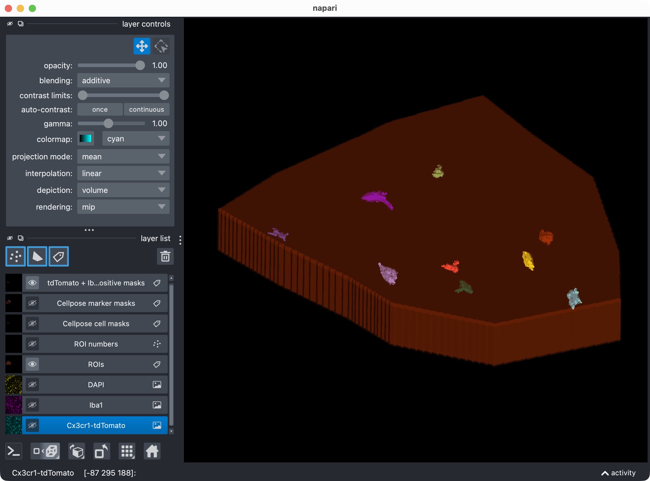
The 3D multi-channel image stack with the raw microglia (magenta), Iba1 (cyan), and DAPI (yellow) channels shown in Napari. Top shows 2D representation, bottom shows 3D representation. The DAPI channel is used for anatomical orientation but not segmented in this tutorial. The microglia channel is segmented with Cellpose, while the Iba1 channel is segmented with Otsu thresholding. The tutorial also demonstrates how to use napari for manual editing of the segmented label layers, and how to reanalyze those edits with CellColoc’s reanalysis function.
Note
In the current script, the DAPI channel is loaded and visualized but not yet segmented for occupancy or third-marker positivity. The core package supports such analyses in general, but this particular tutorial focuses on the two-channel microglia-versus-Iba1 colocalization task.
The same structure can be reused for other 3D multichannel datasets by adapting the path selection, channel assignment, display names, and segmentation settings.
How to use this tutorial
The associated user script
user_scripts/nb_microglia_3D_user_script.ipynb
is organized in cells, reflecting the structure of this tutorial. The same
accounts for the alternative Python script (there: # %% cells)
user_scripts/microglia_3D_user_script.py
The recommended way to follow this tutorial is:
open
user_scripts/nb_microglia_3D_user_script.ipynboruser_scripts/microglia_3D_user_script.py,run the cells from top to bottom,
adjust only the configuration values that are relevant for your own data.
The subsections below follow the same order as the script cells.
Imports and package bootstrap
The first cell imports the public CellColoc API, napari, NumPy, and
dataclasses.replace:
# get the project root for accessing the example dataset which is
# located in the parent folder of the user_scripts folder:
from pathlib import Path
PROJECT_ROOT = Path(__file__).resolve().parents[1]

# import relevant CellColoc functions for this script:
from cellcoloc import (
    CellposeModelConfig,
    ChannelConfig,
    ColocalizationConfig,
    DisplayNames,
    RuntimeConfig,
    create_full_image_roi_labels,
    create_roi_drawing_viewer,
    export_analysis_outputs,
    load_analysis_images,
    load_roi_labels,
    refine_run_result_from_cellpose_cache,
    run_roi_cellpose_colocalization,
    save_roi_labels_from_shapes,
    show_analysis_results,
    try_load_roi_labels,
    analyze_existing_masks,
    extract_label_masks_from_viewer)

# additional packages:
import napari
import numpy as np
from dataclasses import replace
What this cell does:
locates the repository root via
PROJECT_ROOT,imports all interactive analysis helpers needed by this workflow,
imports napari for ROI drawing, result inspection, and manual mask editing,
imports
replacefor building temporary refinement configurations without changing the original base settings.
Project settings
The project settings cell contains the full configuration for this workflow:
# define path to the dataset file relative to the project root:
DATA_DIR = PROJECT_ROOT / "example_data" / "microglia_3D"
# "glob" all image files in the directory:
DATA_PATHS = sorted(DATA_DIR.glob("*"))
allowed_extensions = [".czi", ".tif", ".tiff", ".ome.tif", ".ome.tiff"]
DATA_PATHS = [p for p in DATA_PATHS if p.suffix.lower() in allowed_extensions]
# remove .-prefixed hidden files that some operating systems create:
DATA_PATHS = [p for p in DATA_PATHS if not p.name.startswith(".")]

# define the channel configuration for this dataset:
CHANNEL_CONFIG = ChannelConfig(
    cell_channel=0,
    marker_channel=1,
    optional_region_channel=2)

# define display names for the channels and result layers:
DISPLAY_NAMES = DisplayNames(
    cell="Cx3cr1-tdTomato",
    marker="Iba1",
    optional_region="DAPI",
    positive_cells="tdTomato + Iba1 positive masks")

# optional: define the voxel scale in ZYX (for 3D) or YX (for 2D) order.
# Set this to None to use the voxel scale from the OME metadata, if available.
#VOXEL_SCALE_ZYX = (1.0, 0.6239258, 0.6239258) # CellColoc allows both ZYX and YX even for 2D data.
VOXEL_SCALE_ZYX = None#(1.0, 0.6239258, 0.6239258)

# define the Cellpose model configuration for the cell and marker segmentation:
CELL_MODEL_CONFIG = CellposeModelConfig(
    model_name_or_path="cpsam",     # 'cpsam' for cellpose 4, 'cty3', 'cyto2' or 'nuclei' for cellpose 3
    segmentation_method="cellpose", # 'cellpose' or: 'otsu', 'li', or 'percentile' for marker segmentation
    diameter=None,                  # if None, Cellpose will estimate the diameter from the data. Adjust if you know the expected cell/nuclei size in pixels.
    z_crop=None,                    # optional global analysis z-crop as (start, stop); applies to all channels and all ROIs
    anisotropy=True,                # Cellpose anisotropy correction based on the voxel scale z/y ratio; set to False/True to disable/enable
    flow3d_smooth=3,                # Gaussian smoothing for 3D flow fields; int, default: 0, range: 0-10
    prefilter="gaussian",           # available options: "gaussian", "laplacian_of_gaussian"/"log", "median", None
        prefilter_sigma_xy=0.8,     # Gaussian prefilter sigma in xy; float, default: 0.0 (no prefilter), range: 0.0-10.0
        prefilter_sigma_z=0.0,      # Gaussian prefilter sigma in z; float, default: 0.0 (no prefilter), range: 0.0-10.0
        prefilter_median_size_xy=3, # Median prefilter size in xy; int, default: 0 (no prefilter), range: 0-10
        prefilter_median_size_z=3,  # Median prefilter size in z; int, default: 0 (no prefilter), range: 0-10
    postfilters=None,                   # available options: "min_intensity", "local_contrast", "bright_pixel_support", None
        min_intensity_measure="mean",   # measure for min intensity postfilter; available options: "mean", "max", "median"
        min_intensity_threshold=None,   # threshold for min intensity postfilter; float, no default, range depends on the image data
        local_contrast_k=1.0,           # k for local contrast postfilter; float, default: 1.0, range: 0.0-10.0
        local_contrast_shell_inner_radius=1, # local contrast shell inner radius in pixels; int, default: 1, range: 0-10
        local_contrast_shell_outer_radius=4, # local contrast shell outer radius in pixels; int, default: 4, range: 0-20
        bright_pixel_measure="count",   # measure for bright pixel support postfilter; available options: "count", "fraction"
        bright_pixel_threshold=None,    # threshold for bright pixel support postfilter; float, no default, range depends on the image data
        bright_pixel_min_count=None,    # minimum count for bright pixel support postfilter; int, no default, range depends on the image data
        bright_pixel_min_fraction=None, # minimum fraction for bright pixel support postfilter; float, no default, range depends on the image data
    cellprob_threshold=1.5,         # threshold for the cell probability map, between -6 and 6, where higher values lead to fewer cells (default: 0.0)
    flow_threshold=0.4,             # quality threshold; After mask generation, Cellpose checks whether the flows reconstructed from the mask are
                                    # consistent with the flows predicted by the network. The mean squared error between the two is used as the flow
                                    # error; masks with an error that is too large are discarded. The default value is 0.4.
                                    # The higher, the more tolerant the algorithm is, i.e. more cells but also more false positives.
    )

# define the Cellpose model configuration for the cell and marker segmentation:
MARKER_MODEL_CONFIG = CellposeModelConfig(
    model_name_or_path="cpsam",
    segmentation_method="otsu",
    anisotropy=True,
    flow3d_smooth=3,
    prefilter="laplacian_of_gaussian",
        prefilter_sigma_xy=2.0,
        prefilter_sigma_z=0.1,
        prefilter_median_size_xy=3,
        prefilter_median_size_z=3,
    postfilters=None,
        min_intensity_measure="mean",
        min_intensity_threshold=None,
        local_contrast_k=1.0,
        local_contrast_shell_inner_radius=1,
        local_contrast_shell_outer_radius=4,
        bright_pixel_measure="count",
        bright_pixel_threshold=None,
        bright_pixel_min_count=None,
        bright_pixel_min_fraction=None,
    cellprob_threshold=0,
    flow_threshold=0.4)

# define the colocalization configuration:
COLOCALIZATION_CONFIG = ColocalizationConfig(
    min_cell_voxels=50,
    overlap_fraction_threshold=0.02,
    min_overlap_voxels=10)

# define the runtime configuration:
RUNTIME_CONFIG = RuntimeConfig(
    draw_rois=True,
    process_rois=True,
    open_results=True,
    use_gpu=True,
    crop_for_testing=None,
    image_loading_mode="memap",  # available options: "memory", "memap"
)

USE_FULL_IMAGE_AS_SINGLE_ROI = False
REUSE_EXISTING_ROI_MASK_IF_AVAILABLE = True
INITIAL_RESULT_LAYER_KEYS = [ # controls which layers are shown in napari after the initial analysis run;
    "cell_image",
    "marker_image",
    "optional_region_image",
    "rois",
    "roi_numbers",
    "cell_masks",
    "marker_masks",
    "positive_cells"]
REFINEMENT_RESULT_LAYER_KEYS = [ # controls which layers are shown in napari after the optional refinement based on cached Cellpose outputs;
    "cell_masks",
    "marker_masks",
    "positive_cells",
    "rois"]

# select the dataset file to analyze if there are multiple files in the input directory:
print("Detected input files:")
for data_path in DATA_PATHS:
    print(f" - {data_path.name}")
SELECTED_FILE_NAME = DATA_PATHS[0].name
DATA_PATH = DATA_DIR / SELECTED_FILE_NAME
print(f"Selected file for analysis:\n{DATA_PATH}")
This is the most important cell for adapting the tutorial to your own 3D data.
Input-file discovery and selection
Instead of hardcoding one single filename, the script scans
example_data/microglia_3D/ for microscopy files and lets you select one of
them through:
SELECTED_FILE_NAME = DATA_PATHS[0].name
To analyze a different file in the same folder, simply change this assignment to another detected entry.
Channel assignment and display names
CHANNEL_CONFIG defines the raw-channel meaning:
cell_channel=0marker_channel=1optional_region_channel=2
DISPLAY_NAMES controls how these channels and result layers appear in
napari.
Although optional_region_channel is set to the DAPI channel, the current
script does not yet pass an optional_region_model_config into the main run
function. This means DAPI is available for display, but the present script does
not perform third-channel segmentation or third-channel positivity analysis.
Voxel scale
VOXEL_SCALE_ZYX can be provided explicitly or set to None:
Nonetells CellColoc to read physical voxel sizes from OMIO metadata if possible,otherwise the fallback path uses
(1.0, 1.0, 1.0).
For 3D datasets you would normally provide or infer a full (Z, Y, X) scale,
but CellColoc now also accepts a shorter (Y, X) tuple for 2D-oriented
workflows.
Cell-channel segmentation configuration
CELL_MODEL_CONFIG controls segmentation of the primary microglia channel.
This script uses:
segmentation_method="cellpose"model_name_or_path="cpsam"diameter=None
In addition, it demonstrates several 3D-specific options:
z_crop: optional global analysis z interval applied consistently to all channels and all ROIs.anisotropy=True: let CellColoc derive the Cellpose anisotropy factor automatically from the voxel-size ratio when appropriate.flow3d_smooth=3: smooth 3D Cellpose flows before mask generation.
It also demonstrates optional pre- and post-processing hooks:
prefilterand associated sigma or median-size parameters,postfiltersand their associated intensity or contrast parameters.
These options are particularly useful for suppressing false positive somata, weak edge artifacts, or small disconnected objects in 3D stacks.
Marker-channel segmentation configuration
MARKER_MODEL_CONFIG demonstrates that the marker channel does not have to
use Cellpose.
In this script, the Iba1 channel is segmented with:
segmentation_method="otsu"a
laplacian_of_gaussianprefilter
This is a good illustration of CellColoc’s mixed-backend design: one channel can use neural-network segmentation while another uses a classical threshold-based method in the same analysis run.
Colocalization settings
COLOCALIZATION_CONFIG controls how overlap becomes a positive or negative
cell call.
The key parameters are:
min_cell_voxelsmin_overlap_voxelsoverlap_fraction_threshold
Together they implement the object-based positivity rule described in the overview documentation.
Runtime settings
RUNTIME_CONFIG controls runtime behavior. In this 3D tutorial, two
settings are especially important:
use_gpu=True: relevant when Cellpose is run on the 3D cell channel.image_loading_mode="memap": use OMIO’s disk-backed cache instead of materializing the full raw image eagerly in memory.
For large stacks, "memap" is often the better default because it reduces
the memory burden of raw-image loading.
Whole-image versus ROI mode
This script defaults to ROI-based analysis:
USE_FULL_IMAGE_AS_SINGLE_ROI = FalseREUSE_EXISTING_ROI_MASK_IF_AVAILABLE = True
This means CellColoc will:
reuse an already saved ROI label mask when it exists,
otherwise open napari for ROI drawing.
You can switch to whole-image analysis by setting:
USE_FULL_IMAGE_AS_SINGLE_ROI = True
Napari result-layer selections
The script defines two logical layer lists:
INITIAL_RESULT_LAYER_KEYSREFINEMENT_RESULT_LAYER_KEYS
These determine which layers are shown or refreshed in napari after the initial run and after refinement. This keeps the viewer manageable during iterative work and avoids re-adding every layer on each update.
Load the analysis channels
The next cell loads the selected stack:
loaded_images = load_analysis_images(
    source_path=DATA_PATH,
    channel_config=CHANNEL_CONFIG,
    voxel_scale_zyx=VOXEL_SCALE_ZYX,
    crop_for_testing=RUNTIME_CONFIG.crop_for_testing,
    image_loading_mode=RUNTIME_CONFIG.image_loading_mode)
print(f"Results directory:\n{loaded_images.paths.results_dir}")
existing_roi_labels = None
if REUSE_EXISTING_ROI_MASK_IF_AVAILABLE:
    existing_roi_labels = try_load_roi_labels(loaded_images.paths.roi_mask_path)
This step:
opens the selected microscopy file through OMIO,
extracts the configured channels as analysis volumes,
resolves voxel size,
prepares the standardized results directory,
optionally looks for an already saved ROI mask.
Because REUSE_EXISTING_ROI_MASK_IF_AVAILABLE is enabled in this script, the
loader is followed immediately by a lookup for loaded_images.paths.roi_mask_path.
For large stacks, you can additionally reduce the problem size temporarily with
RUNTIME_CONFIG.crop_for_testing = (slice(0, 16), slice(100, 300), slice(100, 300))
This crop is defined in ZYX order.
Optional: Draw ROIs interactively in napari
The next cell controls whether ROIs are drawn or skipped:
if USE_FULL_IMAGE_AS_SINGLE_ROI:
    print("Whole-image mode is enabled. ROI drawing is skipped.")
elif existing_roi_labels is not None:
    print("An existing ROI mask was found and will be reused. ROI drawing is skipped.")
elif RUNTIME_CONFIG.draw_rois:
    roi_viewer, shapes_layer = create_roi_drawing_viewer(
        loaded_images=loaded_images,
        display_names=DISPLAY_NAMES)
    print("Draw ROIs in napari and close the window. Then run the next cell.")
    napari.run()
else:
    print("ROI drawing is disabled. The next cell will load an existing ROI mask from disk.")
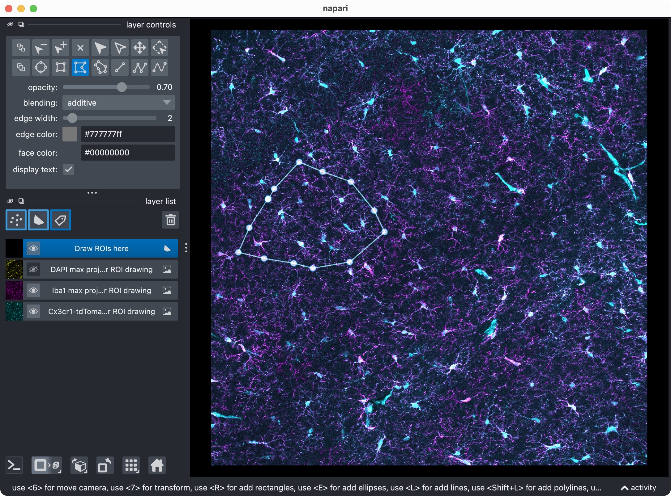
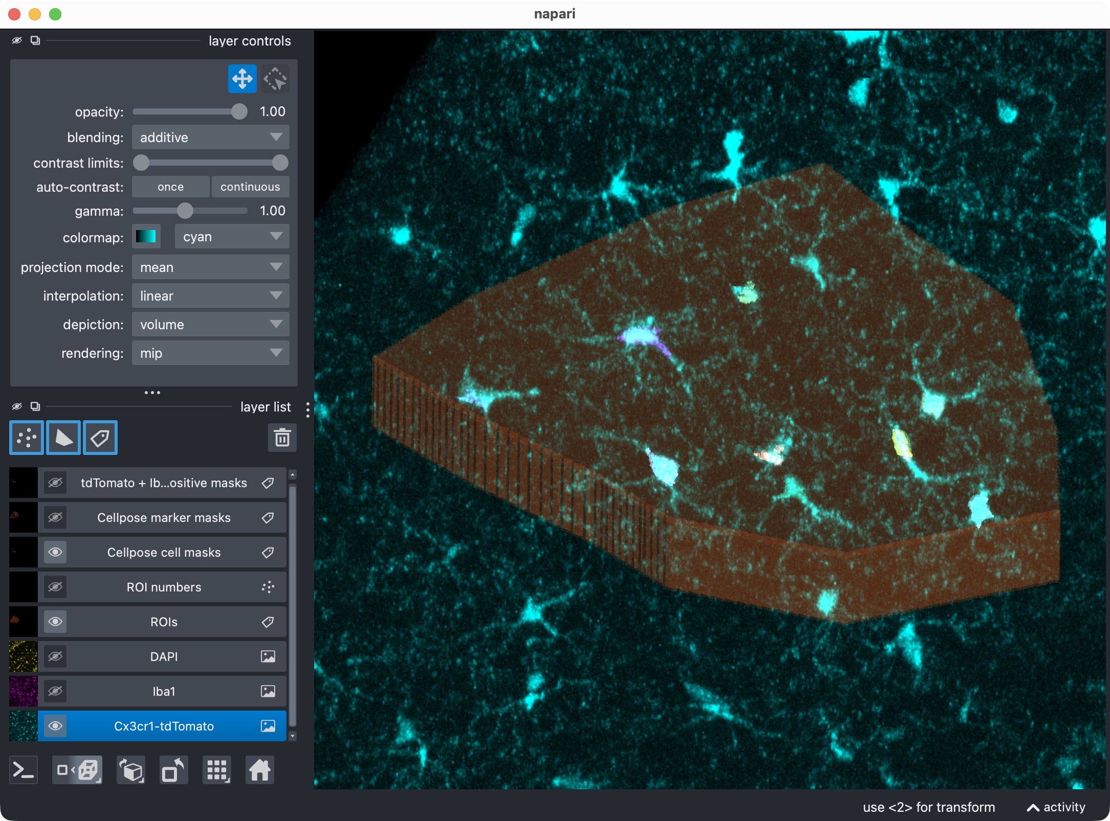
The three image layers (=channels) and the shape layer. Napari allows to draw any arbitrary 2D ROI shapes on top of the image layers. In this tutorial, we draw one ROI in 2D. CellColoc will then apply that ROI across the z dimension for the internal analysis (unless no z-cropping is defined), but the original 3D shape of the ROI is defined in 2D. The ROI drawing step is optional and can be skipped by setting USE_FULL_IMAGE_AS_SINGLE_ROI = True. In that case, the whole image will be treated as one single ROI, and no shape layers will be added to the viewer.
The logic is:
whole-image mode skips ROI drawing,
otherwise an existing ROI mask is reused when found,
otherwise napari opens for interactive ROI drawing.
As in the 2D tutorial, ROIs are drawn in 2D and then applied across the stack in z for the internal analysis.
Optional: Save drawn ROIs or load an existing ROI mask
The next cell resolves the actual ROI label image:
if USE_FULL_IMAGE_AS_SINGLE_ROI:
    roi_labels_2d = create_full_image_roi_labels(loaded_images.cell_image.shape[1:])
elif existing_roi_labels is not None:
    roi_labels_2d = existing_roi_labels
elif RUNTIME_CONFIG.draw_rois:
    roi_labels_2d = save_roi_labels_from_shapes(
        shapes_layer=shapes_layer,
        output_path=loaded_images.paths.roi_mask_path,
        image_shape_yx=loaded_images.cell_image.max(axis=0).shape,
        scale_yx=loaded_images.voxel_scale_zyx[1:])
else:
    roi_labels_2d = load_roi_labels(loaded_images.paths.roi_mask_path)

roi_ids = np.unique(roi_labels_2d)
roi_ids = roi_ids[roi_ids != 0]
print(f"ROI ids: {roi_ids}")
result_viewer = None
Supported modes are:
one full-image ROI,
newly drawn ROIs from napari,
or a previously saved ROI label mask.
After this step, roi_labels_2d is the final ROI definition used by all
later analysis steps, and the script prints the detected ROI IDs.
Run the ROI-wise segmentation and colocalization analysis
The next cell performs the actual 3D segmentation and colocalization run:
run_result = run_roi_cellpose_colocalization(
    loaded_images=loaded_images,
    roi_labels_2d=roi_labels_2d,
    cell_model_config=CELL_MODEL_CONFIG,
    marker_model_config=MARKER_MODEL_CONFIG,
    colocalization_config=COLOCALIZATION_CONFIG,
    runtime_config=RUNTIME_CONFIG,
    optional_region_result=None)
print("Initial analysis finished. "
      f"Overview rows: {len(run_result.tables.overview)}, "
      f"summary rows: {len(run_result.tables.summary)}.")
What happens here:
each ROI is processed separately,
the microglia channel is segmented with Cellpose,
the Iba1 channel is segmented with Otsu thresholding,
per-cell overlaps are computed,
marker-positive cells are classified,
result tables and derived masks are assembled.
The returned run_result stores:
the current label masks,
the detailed, summary, and overview tables,
the current analysis z bounds,
optional Cellpose refinement caches for later threshold-only rebuilding.
Visualize the result in napari
The next cell opens the current result in napari:
if RUNTIME_CONFIG.open_results:
    result_viewer = None
    result_viewer = show_analysis_results(
        loaded_images=loaded_images,
        roi_labels_2d=roi_labels_2d,
        run_result=run_result,
        display_names=DISPLAY_NAMES,
        optional_region_result=None,
        viewer=result_viewer,
        layers_to_show=INITIAL_RESULT_LAYER_KEYS,
        replace_existing_layers=True,
        show_optional_region_image=True)

    print(f"Inspecting visualization for:\n{SELECTED_FILE_NAME}")
    napari.run()
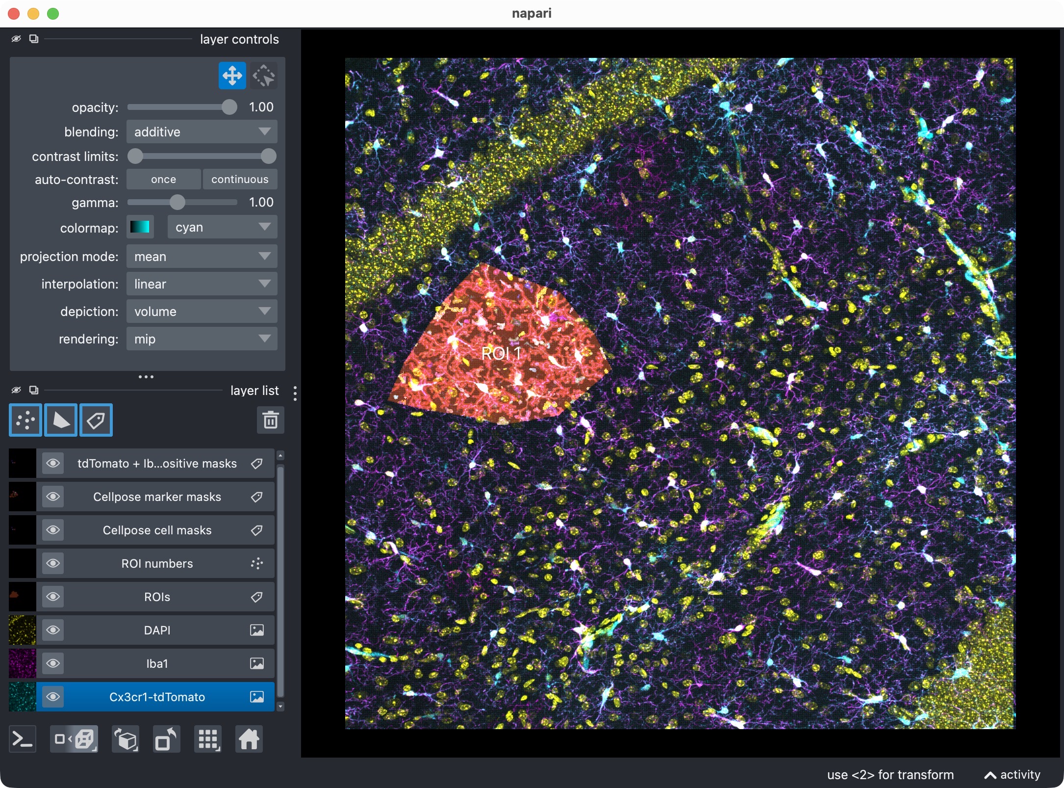
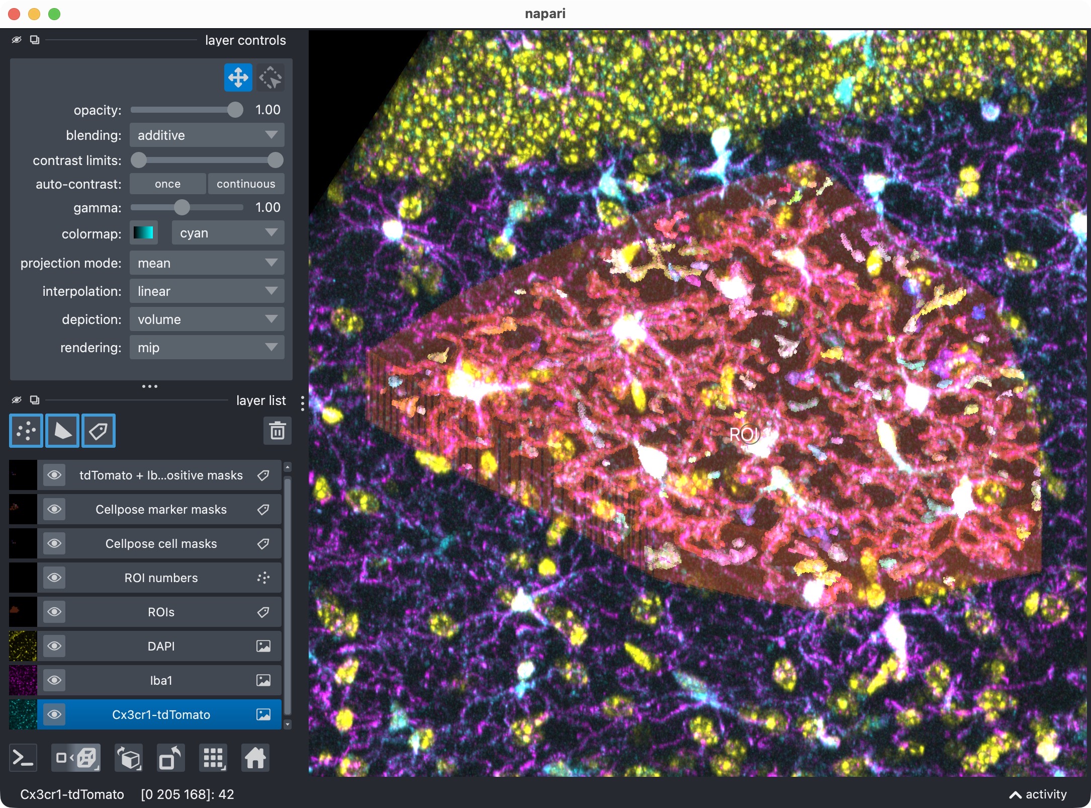
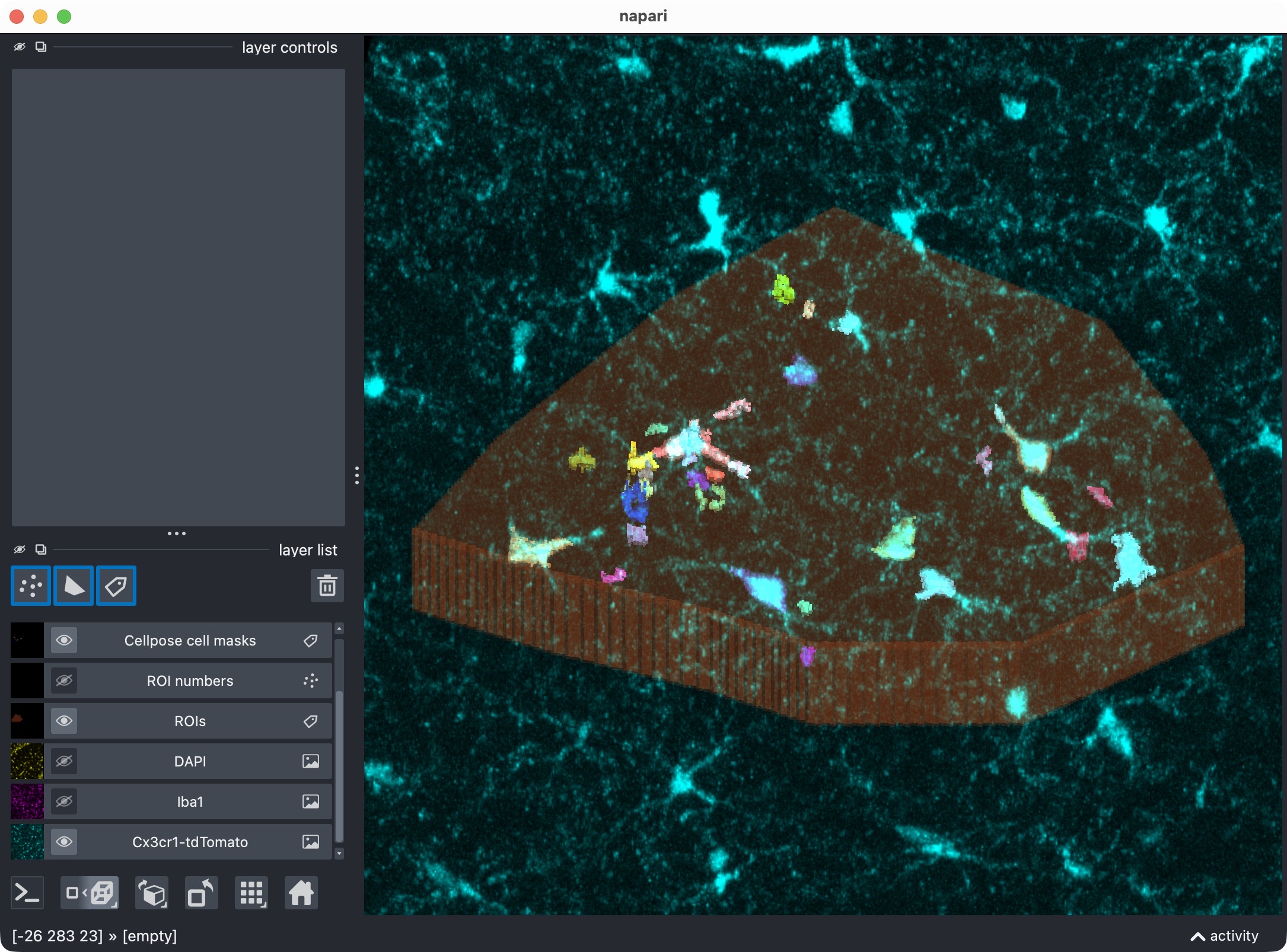
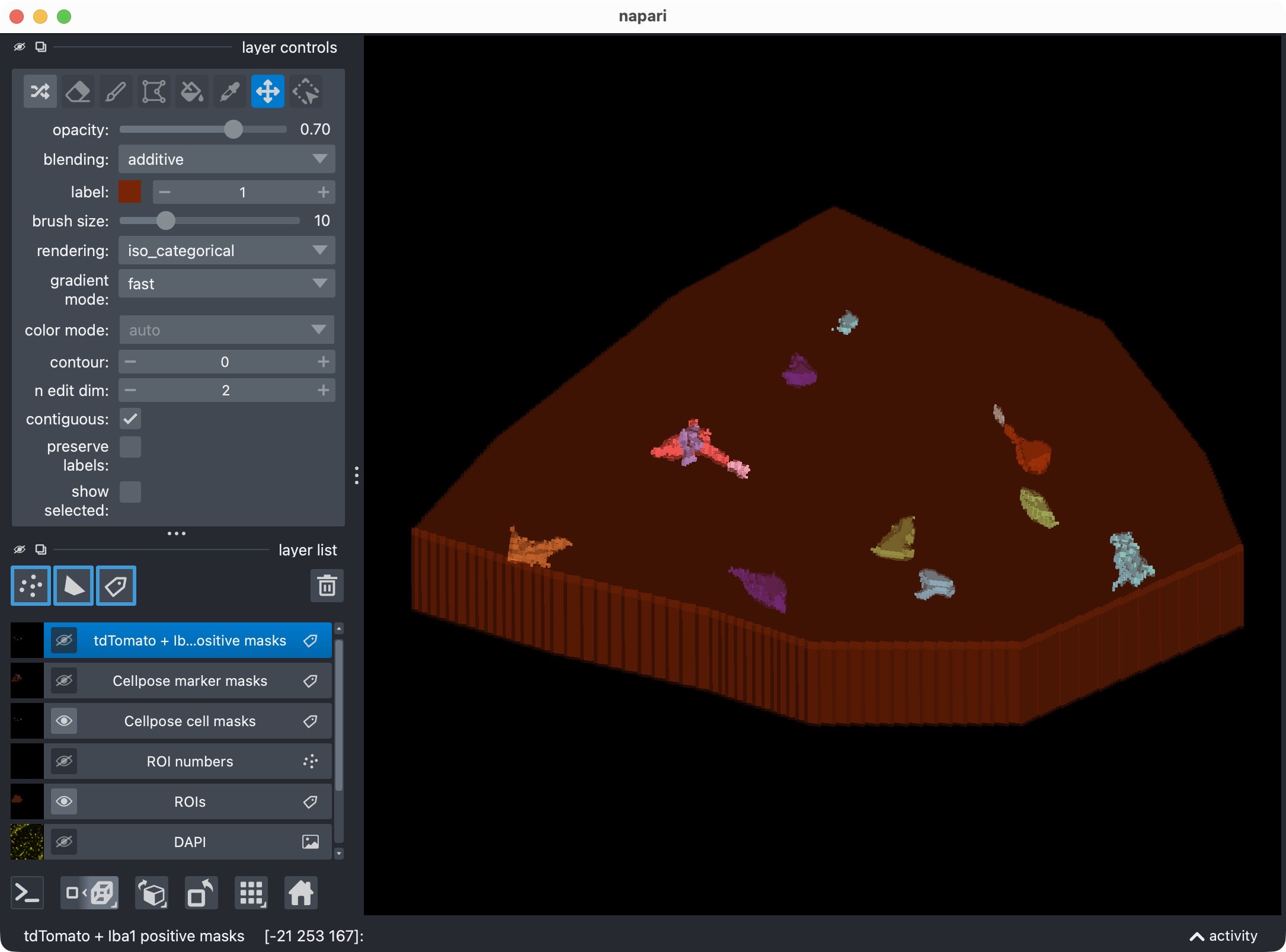
Results of the initial analysis run shown in napari (top: 2D view, bottom: 3D zoomed view of the analyzed ROI). The raw image channels are shown together with the derived label layers for ROIs, cell masks, marker masks, and positive-cell masks. This viewer is the main interactive checkpoint of the 3D workflow.
This viewer is the main interactive checkpoint of the 3D workflow. It can show:
the raw microglia channel,
the raw Iba1 channel,
the DAPI channel for orientation,
ROI labels and ROI numbers,
segmented cell masks,
segmented marker masks,
the derived positive-cell mask.
Because the script reuses result_viewer later on, this is also the viewer
you can edit manually before the manual reanalysis step at the end.
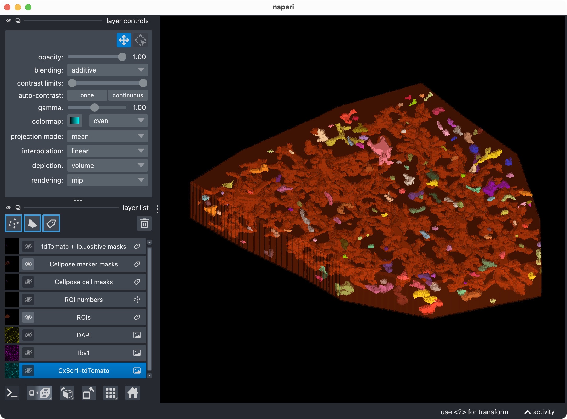
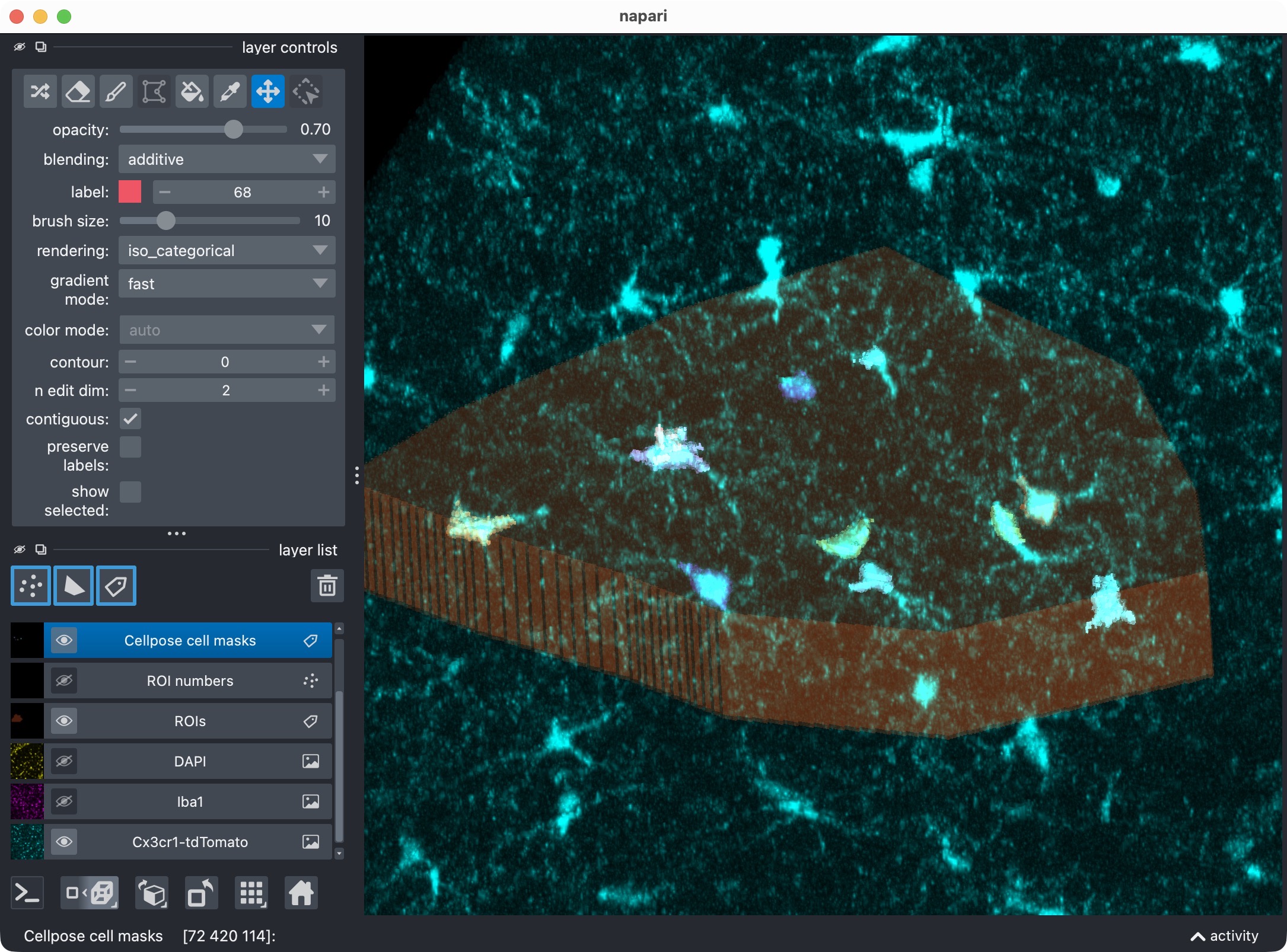
Inspecting the microglia channel results. Top: Overlay of raw microglia channel (magenta) and segmented cell mask. Bottom: 3D rendering of the same. This is a good time to check whether the Cellpose segmentation worked well across the z dimension, or whether some slices should be excluded from the analysis with a global z-crop before refinement. Also, note that the segmentation of the microglia channel is not perfect: We miss at least one microglial soma in the upper center. In the next refinement step, we will see how to use the Cellpose cache to adjust the cell-channel thresholds and postfilters in order to recover that missed cell without having to rerun Cellpose from scratch on the full 3D stack.
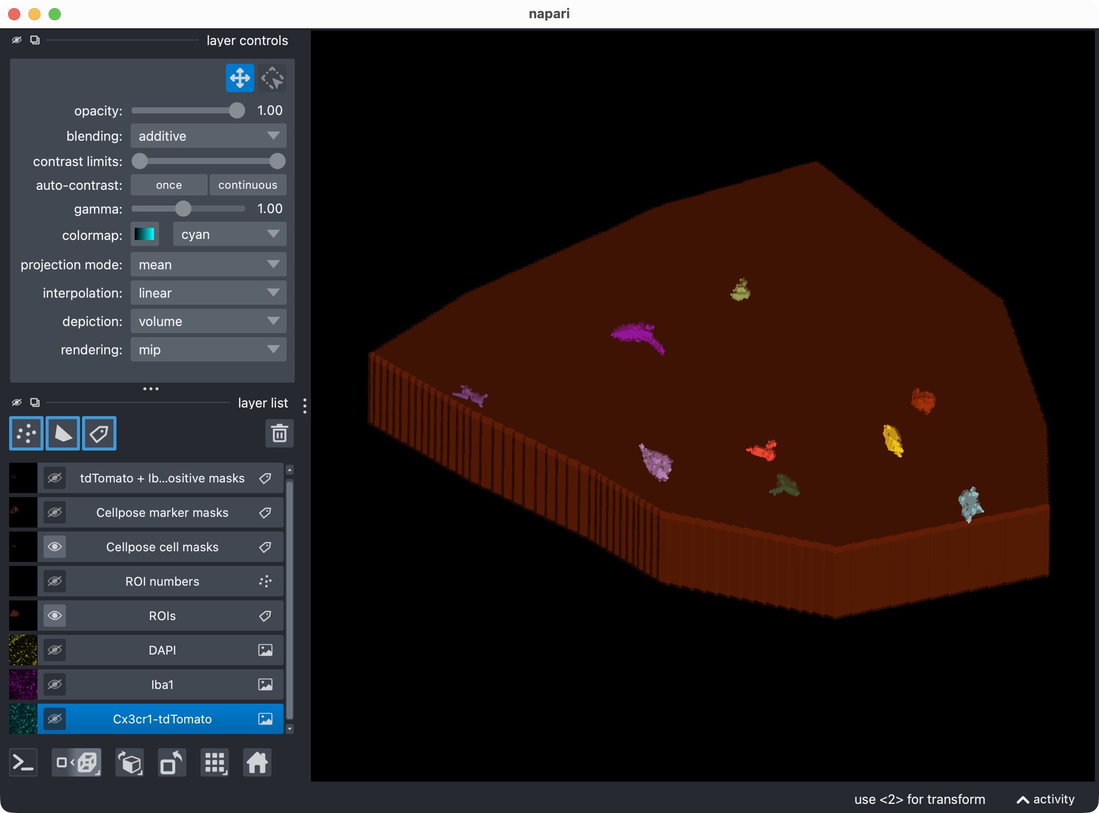
Top: The segmentation mask of the Iba1 marker channel. Bottom: The resulting colocalization calls. The positive-cell mask shows the microglia that were classified as Iba1-positive based on their overlap with the marker mask. In this example, we have chosen to segment the marker channel with Otsu thresholding, which is not perfect. You may see that the segmentation of the marker channel is resulted into too broad and thick cell processes, which can lead to some false positive colocalization calls in the positive-cell mask. However, for demonstration purposes, this is still a good result as we are at first glance interested in the overall workflow and the overall Iba1-positivity rate of the microglia, rather than in the perfect segmentation of every single cell process in this channel. For a real project, you would of course want to optimize the marker-channel segmentation and the colocalization settings to get the best possible result for your specific data and question.
Optionally set or update a global z-crop for subsequent refinement
This cell is specific to the 3D workflow:
REFINEMENT_ANALYSIS_Z_CROP = (5,20)
#REFINEMENT_ANALYSIS_Z_CROP = None
# Example: (5, 24) or None
# `None` keeps the current analysis z range unchanged.
# A tuple such as `(z_start, z_stop)` restricts all subsequent internal
# refinement calculations to that z interval for all channels and all ROIs.
if REFINEMENT_ANALYSIS_Z_CROP is None:
    print(f"No refinement z-crop requested. Subsequent refinement will keep the "
          f"current analysis z range: {run_result.analysis_z_bounds}.")
else:
    print(f"Subsequent refinement will use this global analysis z-crop:\n"
          f"{REFINEMENT_ANALYSIS_Z_CROP}")
Its purpose is didactic and practical:
you first inspect the full 3D result,
then decide whether the upper or lower slices should be excluded from the refinement and final quantification,
and finally rerun the analysis logic in that restricted z interval.
Set:
REFINEMENT_ANALYSIS_Z_CROP = Noneto keep the current analysis range,or a tuple such as
(5, 20)to restrict subsequent internal calculations to that z interval.
This crop affects all channels and all ROIs consistently during the following refinement step.
Optionally refine results and visualize the updated result
The next cell performs cache-based refinement and then refreshes the napari layers:
REFINE_WITH_CACHED_CELLPOSE_OUTPUTS = True

REFINED_CELL_CELLPROB_THRESHOLD = CELL_MODEL_CONFIG.cellprob_threshold- 3.0 # - 0.9
REFINED_CELL_FLOW_THRESHOLD = CELL_MODEL_CONFIG.flow_threshold-0.2 # 0.1

REFINED_MARKER_CELLPROB_THRESHOLD = -3#4.5
REFINED_MARKER_FLOW_THRESHOLD = 0.4#0.8

REFINED_CELL_POSTFILTERS = ["min_intensity", "bright_pixel_support", "local_contrast"] # available options: "min_intensity", "local_contrast", "bright_pixel_support", None
REFINED_CELL_MIN_INTENSITY_MEASURE = "max"
REFINED_CELL_MIN_INTENSITY_THRESHOLD = 250
REFINED_CELL_LOCAL_CONTRAST_K = 4
REFINED_CELL_LOCAL_CONTRAST_SHELL_INNER_RADIUS = 1.0
REFINED_CELL_LOCAL_CONTRAST_SHELL_OUTER_RADIUS = 10
REFINED_CELL_BRIGHT_PIXEL_MEASURE = "fraction"
REFINED_CELL_BRIGHT_PIXEL_THRESHOLD = 110
REFINED_CELL_BRIGHT_PIXEL_MIN_COUNT = None
REFINED_CELL_BRIGHT_PIXEL_MIN_FRACTION = 0.08

#REFINED_MARKER_POSTFILTERS = ["min_intensity", "bright_pixel_support", "local_contrast"] #"local_contrast" # available options: "min_intensity", "local_contrast", "bright_pixel_support", None
REFINED_MARKER_POSTFILTERS = ["min_intensity", "bright_pixel_support", "local_contrast"]
REFINED_MARKER_MIN_INTENSITY_MEASURE = "max"
REFINED_MARKER_MIN_INTENSITY_THRESHOLD = 250
REFINED_MARKER_LOCAL_CONTRAST_K = 1
REFINED_MARKER_LOCAL_CONTRAST_SHELL_INNER_RADIUS = 1.0
REFINED_MARKER_LOCAL_CONTRAST_SHELL_OUTER_RADIUS = 4
REFINED_MARKER_BRIGHT_PIXEL_MEASURE = "fraction"
REFINED_MARKER_BRIGHT_PIXEL_THRESHOLD = 120
REFINED_MARKER_BRIGHT_PIXEL_MIN_COUNT = None
REFINED_MARKER_BRIGHT_PIXEL_MIN_FRACTION = 0.09

effective_refinement_z_crop = (
    CELL_MODEL_CONFIG.z_crop if REFINEMENT_ANALYSIS_Z_CROP is None else REFINEMENT_ANALYSIS_Z_CROP)

if REFINE_WITH_CACHED_CELLPOSE_OUTPUTS:
    refined_cell_model_config = replace(
        CELL_MODEL_CONFIG,
        z_crop=effective_refinement_z_crop,
        postfilters=REFINED_CELL_POSTFILTERS,
        min_intensity_measure=REFINED_CELL_MIN_INTENSITY_MEASURE,
        min_intensity_threshold=REFINED_CELL_MIN_INTENSITY_THRESHOLD,
        local_contrast_k=REFINED_CELL_LOCAL_CONTRAST_K,
        local_contrast_shell_inner_radius=REFINED_CELL_LOCAL_CONTRAST_SHELL_INNER_RADIUS,
        local_contrast_shell_outer_radius=REFINED_CELL_LOCAL_CONTRAST_SHELL_OUTER_RADIUS,
        bright_pixel_measure=REFINED_CELL_BRIGHT_PIXEL_MEASURE,
        bright_pixel_threshold=REFINED_CELL_BRIGHT_PIXEL_THRESHOLD,
        bright_pixel_min_count=REFINED_CELL_BRIGHT_PIXEL_MIN_COUNT,
        bright_pixel_min_fraction=REFINED_CELL_BRIGHT_PIXEL_MIN_FRACTION)
    refined_marker_model_config = replace(
        MARKER_MODEL_CONFIG,
        z_crop=effective_refinement_z_crop,
        postfilters=REFINED_MARKER_POSTFILTERS,
        min_intensity_measure=REFINED_MARKER_MIN_INTENSITY_MEASURE,
        min_intensity_threshold=REFINED_MARKER_MIN_INTENSITY_THRESHOLD,
        local_contrast_k=REFINED_MARKER_LOCAL_CONTRAST_K,
        local_contrast_shell_inner_radius=REFINED_MARKER_LOCAL_CONTRAST_SHELL_INNER_RADIUS,
        local_contrast_shell_outer_radius=REFINED_MARKER_LOCAL_CONTRAST_SHELL_OUTER_RADIUS,
        bright_pixel_measure=REFINED_MARKER_BRIGHT_PIXEL_MEASURE,
        bright_pixel_threshold=REFINED_MARKER_BRIGHT_PIXEL_THRESHOLD,
        bright_pixel_min_count=REFINED_MARKER_BRIGHT_PIXEL_MIN_COUNT,
        bright_pixel_min_fraction=REFINED_MARKER_BRIGHT_PIXEL_MIN_FRACTION)

    run_result = refine_run_result_from_cellpose_cache(
        loaded_images=loaded_images,
        roi_labels_2d=roi_labels_2d,
        run_result=run_result,
        colocalization_config=      COLOCALIZATION_CONFIG,
        cell_model_config=          refined_cell_model_config,
        marker_model_config=        None,#refined_marker_model_config,
        cell_cellprob_threshold=    REFINED_CELL_CELLPROB_THRESHOLD,
        cell_flow_threshold=        REFINED_CELL_FLOW_THRESHOLD,
        marker_cellprob_threshold=  REFINED_MARKER_CELLPROB_THRESHOLD,
        marker_flow_threshold=      REFINED_MARKER_FLOW_THRESHOLD,
        optional_region_result=     None)

    print("Refinement finished. "
          f"Overview rows: {len(run_result.tables.overview)}, "
          f"summary rows: {len(run_result.tables.summary)}.")

    if RUNTIME_CONFIG.open_results:
        result_viewer = show_analysis_results(
            loaded_images=loaded_images,
            roi_labels_2d=roi_labels_2d,
            run_result=run_result,
            display_names=DISPLAY_NAMES,
            optional_region_result=None,
            viewer=result_viewer,
            layers_to_show=REFINEMENT_RESULT_LAYER_KEYS,
            replace_existing_layers=True,
            show_optional_region_image=True)

        print(f"Inspecting refined visualization for:\n{SELECTED_FILE_NAME}")
        napari.run()
else:
    print("Cached Cellpose refinement is disabled for this run.")
This step is especially useful in 3D because a full Cellpose rerun can be costly. The refinement reuses cached network outputs from the initial Cellpose run.
The cell demonstrates several advanced ideas at once:
threshold refinement for the cell channel,
optional postfilter refinement,
optional z-crop refinement,
selective viewer-layer refresh,
and channel-specific refinement control.
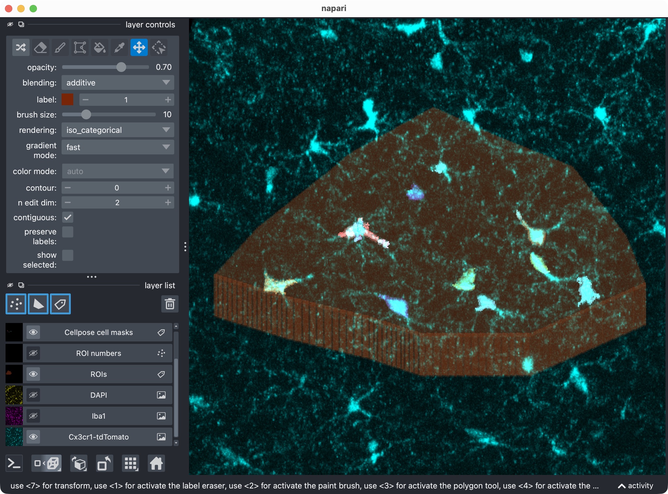
First refinement attempt in order to recover the missed microglial soma in the upper center. In this case, we adjust Cellpose’s cellprob_threshold and flow_threshold to be more permissive, which allows Cellpose to generate a new candidate mask that includes the missed cell. However, the refined thresholds resulted into a too permissive segmentation with many false positives.
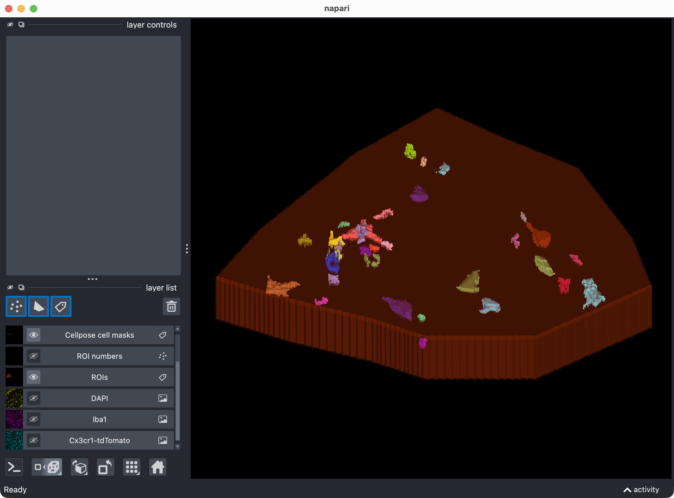
Final refinement attempt in order to recover the missed microglial soma in the upper center, further fine-tuning Cellpose’s cellprob_threshold and flow_threshold. This time, we find a better balance between sensitivity and specificity, which allows us to recover the missed cell while keeping the false positives at a more manageable level. However, some false positives still remain, which is not ideal. In the next step, we will therefore see how to use napari for manual editing of the segmented label layers, and how to reanalyze those edits with CellColoc’s reanalysis function in order to delete some of the false positives while keeping the recovered true positive cell in place.
Channel-selective refinement
In the current script, only the cell channel is actually refined:
marker_model_config=None
inside the call to refine_run_result_from_cellpose_cache(...).
This means:
the cell masks are rebuilt from cached Cellpose outputs using the new cell thresholds and postfilters,
the marker masks are kept unchanged from the previous state.
If you want to refine the marker channel as well, pass
refined_marker_model_config instead of None.
The script exposes several groups of refinement parameters. These let you keep the initial segmentation run unchanged while iteratively exploring better final settings:
Cellpose refinements
These settings control cache-based rebuilding of Cellpose masks:
REFINE_WITH_CACHED_CELLPOSE_OUTPUTS: master switch for the refinement step. If this isFalse, the script keeps the current result unchanged and skips the cache-based rebuilding.REFINED_CELL_CELLPROB_THRESHOLD: updated Cellpose cell-probability threshold for the cell channel.REFINED_CELL_FLOW_THRESHOLD: updated flow-consistency threshold for the cell channel.REFINED_MARKER_CELLPROB_THRESHOLD: nominal marker-channel Cellpose probability threshold.REFINED_MARKER_FLOW_THRESHOLD: nominal marker-channel flow threshold.
How to interpret these values:
lower
cellprob_threshold: generally more permissive, often yielding more candidate masks, including weaker or partially missed cells,higher
cellprob_threshold: more conservative, usually yielding fewer but cleaner masks,higher
flow_threshold: more tolerant with respect to flow inconsistency, which can keep masks that would otherwise be discarded,lower
flow_threshold: stricter, which can remove questionable masks but may also discard difficult true positives.
In practice, these thresholds are often tuned together:
if a true cell is missing, you may try lowering
REFINED_CELL_CELLPROB_THRESHOLDfirst,if Cellpose proposes a mask but seems to discard it too aggressively, you may then increase
REFINED_CELL_FLOW_THRESHOLDslightly,if too many false positives appear, move the settings back toward stricter values.
Even when the marker channel is not actively refined in this script, the marker threshold variables are still shown for completeness and to make it easy to switch to marker refinement later.
Postfilters
The script also exposes post-hoc mask cleanup settings for both channels. These are applied after segmentation and are especially useful for removing false positive soma-like artifacts or over-permissive threshold fragments.
General postfilter selector
REFINED_CELL_POSTFILTERSREFINED_MARKER_POSTFILTERS
These can be set to:
None: disable postfiltering,"min_intensity""local_contrast""bright_pixel_support"or a list such as
["min_intensity", "bright_pixel_support", "local_contrast"]
When a list is used, the filters are applied in that exact order.
Minimum intensity threshold min_intensity
Relevant parameters:
REFINED_*_MIN_INTENSITY_MEASUREREFINED_*_MIN_INTENSITY_THRESHOLD
Supported measures are:
"mean""median""max"
Interpretation:
mean: stricter on weak, diffuse masks, but can remove real objects when they are only moderately bright overall,median: more robust to a few outlier pixels and often a good compromise,max: most permissive, because a single bright region can keep an object alive.
This filter asks:
is the signal inside the object strong enough in the original image at all?
Local contrast threshold local_contrast
Relevant parameters:
REFINED_*_LOCAL_CONTRAST_KREFINED_*_LOCAL_CONTRAST_SHELL_INNER_RADIUSREFINED_*_LOCAL_CONTRAST_SHELL_OUTER_RADIUS
Interpretation:
local_contrast_k: controls how much brighter an object must be than its local neighborhood,shell_inner_radiusandshell_outer_radius: define the background shell around the object that is used for comparison.
This filter asks:
is this mask locally object-like, that is, clearly brighter than its immediate surroundings?
It is particularly useful for rejecting masks that sit on flat or noisy background regions without representing a convincing local soma signal.
Bright pixel support bright_pixel_support
Relevant parameters:
REFINED_*_BRIGHT_PIXEL_MEASUREREFINED_*_BRIGHT_PIXEL_THRESHOLDREFINED_*_BRIGHT_PIXEL_MIN_COUNTREFINED_*_BRIGHT_PIXEL_MIN_FRACTION
Supported measures are:
"count""fraction"
Interpretation:
count: require at least a minimum absolute number of bright pixels or voxels,fraction: require that at least a certain fraction of the object is above the chosen brightness threshold.
This filter asks:
does the segmented object contain enough genuinely bright support pixels to look biologically plausible?
This is often especially helpful for removing false-positive soma masks that touch only a few bright process pixels.
Z-cropping
The refinement stage also respects the earlier
REFINEMENT_ANALYSIS_Z_CROP setting.
This means you can:
inspect the full stack first,
then decide to exclude weak or blurry upper/lower slices,
and finally refine only inside that analysis z range.
That is often a very effective last tuning step in 3D datasets because it reduces ambiguity without changing the raw ROI definition in XY.
Taken together, these Cellpose and postfilter settings make the refinement stage a convenient place for final tuning after the first qualitative 3D inspection.
Optionally reanalyze manually edited label layers from napari
The final optional analysis cell lets you treat manual napari edits as the new segmentation truth:
REANALYZE_EDITED_LABELS_FROM_VIEWER = True

"""
In the opened Napari viewer, you can manually edit the Cellpose-generated label layers
(e.g. using the brush, eraser, or other label editing tools) to correct any segmentation
errors. When you are done, execute this cell to extract the edited masks from the viewer.
The colocalization analysis will be re-run based on the edited masks, and the updated results
will be displayed in a new Napari viewer instance.
"""

if REANALYZE_EDITED_LABELS_FROM_VIEWER:
    cell_masks_from_viewer, marker_masks_from_viewer = extract_label_masks_from_viewer(result_viewer)
    run_result = analyze_existing_masks(
        loaded_images=loaded_images,
        roi_labels_2d=roi_labels_2d,
        cell_masks=cell_masks_from_viewer,
        marker_masks=marker_masks_from_viewer,
        colocalization_config=COLOCALIZATION_CONFIG,
        optional_region_result=None,
        cell_refinement_context=run_result.cell_refinement_context,
        marker_refinement_context=run_result.marker_refinement_context,
        analysis_z_bounds=run_result.analysis_z_bounds,
    )

    print(run_result.tables.overview.iloc[:, :3])

    result_viewer = show_analysis_results(
        loaded_images=loaded_images,
        roi_labels_2d=roi_labels_2d,
        run_result=run_result,
        display_names=DISPLAY_NAMES,
        optional_region_result=None,
        viewer=result_viewer,
        layers_to_show=REFINEMENT_RESULT_LAYER_KEYS,
        replace_existing_layers=True,
        show_optional_region_image=True,
    )
    print("Inspect the relabeled result in napari and close the window when finished.")
    napari.run()
else:
    print("Manual label reanalysis from the napari viewer is disabled for this run.")
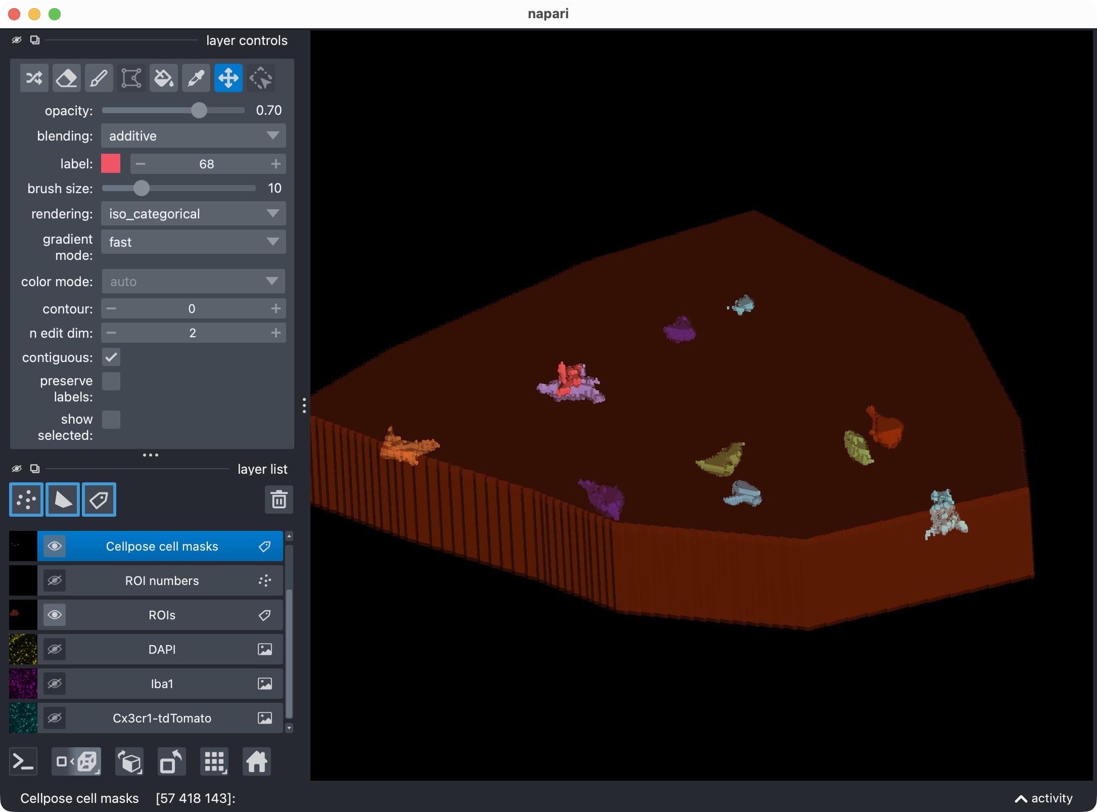
After manually re-assigning falsely split cell compartments and deleting false positive cells using napari’s layer tools, we finally have a clean segmentation of the microglia channel with all true positive cells correctly labeled and most false positives removed. The next step is to let CellColoc treat these manual edits as the new segmentation truth and re-run the colocalization analysis based on those edits. This way, we can keep the manually edited cell masks in place while automatically updating the marker masks, the colocalization calls, and all result tables based on those edits.
Note
Important: First use the napari viewer opened in the previous cell to manually edit the label layers, and after you are done with the editing, then run this cell to let CellColoc extract the edited label arrays from the viewer and re-run the analysis based on those edits. Do not run this cell before you have made your manual edits in napari, otherwise your edits will not be included in the reanalysis.
This is useful when:
Cellpose split one soma into multiple labels,
a false positive should be deleted manually,
or a thresholded marker mask needs local human correction.
The workflow is:
edit the displayed label layers directly in napari,
run this cell,
let CellColoc extract the edited label arrays from the viewer,
recompute the tables based on those edited masks.
Importantly, the script now also passes
analysis_z_bounds=run_result.analysis_z_bounds to the reanalysis function.
This keeps the manual reanalysis consistent with any refinement-time z-crop
that may already have been applied.
Export results
The final cell writes the accepted analysis result to disk:
export_analysis_outputs(
    run_result=run_result,
    paths=loaded_images.paths,
    optional_region_result=None,
)
print("Final results exported.")
Outputs are written to the dataset’s results/ directory and typically
include:
ROI mask,
cell mask,
marker mask,
positive-cell mask,
the detailed CSV table,
and the combined Excel workbook.
As in the 2D workflow, export is intentionally placed at the end so that the saved results represent the final accepted state after any refinement or manual editing. Please refer to the 2D workflow for a detailled description of the results table.
Adapting this tutorial to your own data
To reuse this workflow for your own 3D microscopy project, the most important settings to adapt are:
DATA_DIRandSELECTED_FILE_NAMECHANNEL_CONFIGDISPLAY_NAMESVOXEL_SCALE_ZYXCELL_MODEL_CONFIGMARKER_MODEL_CONFIGCOLOCALIZATION_CONFIGRUNTIME_CONFIGUSE_FULL_IMAGE_AS_SINGLE_ROIandREUSE_EXISTING_ROI_MASK_IF_AVAILABLE
For a practical first pass on a new 3D dataset:
start with one representative file,
use ROI-based analysis rather than whole-image mode when the stack is spatially heterogeneous,
verify voxel scaling and anisotropy handling early,
use
crop_for_testingorimage_loading_mode="memap"if the stack is large,inspect the initial result in napari before enabling any refinement,
use refinement-time z-cropping if upper or lower slices should be excluded,
export only after the 3D result looks correct.